Computer-aided Lyapunov analyses in optimization

Manu Upadhyaya

doi:10.5281/zenodo.23521024

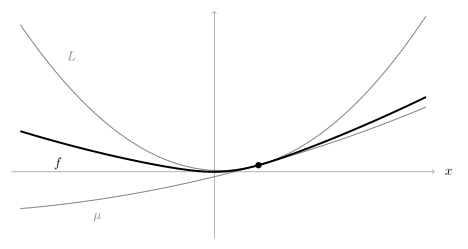
Many convergence proofs for first-order methods in optimization follow a common pattern: construct a Lyapunov function, establish an inequality describing its decrease, and use this inequality to show that a performance measure converges to zero. Within many standard problem classes and prescribed families of Lyapunov functions, these tasks can often be formulated exactly as semidefinite programs (SDPs). Existing solvers can then be used to search numerically for feasible solutions. Convergence analysis itself thus becomes a tractable optimization problem.

Closely related is the performance estimation problem (PEP) methodology, introduced by Drori and Teboulle [DT14]. For many first-order methods and problem classes, the search for a worst-case example can be reformulated as an SDP, giving tight worst-case guarantees [THG17]. The standard PEP methodology is now a mature technology for worst-case analysis, supported by software packages such as PEPit [GMG+24].

However, standard PEP formulations analyze a fixed number of iterations, with the number of variables and constraints typically growing quadratically with this horizon. Deriving closed-form guarantees valid for all iterations can also be challenging. Automated Lyapunov analyses provide a complementary approach: restricting the search to prescribed families of Lyapunov analyses can give smaller SDPs whose number of variables and constraints is independent of the iteration horizon, or grows only linearly with it, facilitating concise, closed-form convergence proofs [TVSL18, TB19, UBTG25, UDGT+26]. A closely related framework uses integral quadratic constraints (IQCs), developed in robust control [MR97], to obtain convergence guarantees through linear matrix inequalities (LMIs) that can be checked by semidefinite programming [LRP16, MSE21]. Although searching over prescribed families of Lyapunov functions may give conservative bounds, these bounds can still match the actual worst-case behavior in many settings.

In this post, we derive the corresponding SDPs explicitly for two examples: an inexact gradient method, for which the Lyapunov function is fixed in advance, and a gradient method with memory, for which we search for a Lyapunov function within a prescribed family. The aim is to explain the main ideas in a simple setting and provide a starting point for analyses of other methods and problem classes. For the first example, we also show how to extract a closed-form proof of a tight convergence guarantee from numerical SDP solutions. In the second example, we show how allowing a more flexible class of Lyapunov functions can give tighter convergence guarantees. This post assumes familiarity with smooth and strongly convex optimization, basic matrix algebra, and Lagrangian duality. On a first reading, the expandable derivations and proofs can be skipped.

1. Problem setting

For simplicity, both examples use the familiar setting of smooth and strongly convex optimization, although the tools developed here apply more broadly. We consider the unconstrained problem

\begin{equation} \label{eq:optimization-problem} \mathop{\text{minimize}}\limits_{x \in \mathbb{R}^d}\; f(x) \end{equation}

where $f:\mathbb{R}^d\to\mathbb{R}$ is differentiable, has an $L$ -Lipschitz continuous gradient (that is, $f$ is $L$ -smooth), and is $\mu$ -strongly convex, with $0<\mu<L$ . We denote this class of functions by $\mathcal{F}_{\mu,L}(\mathbb{R}^d)$ . Equivalently, $f$ satisfies

\begin{equation} \label{eq:quadratic-bounds} (\forall x,y\in\mathbb{R}^{d})\qquad \left[ \begin{aligned} f(x) &\leqslant f(y)+\langle\nabla f(y),x-y\rangle +\tfrac{L}{2}\lVert x-y\rVert^{2},\\ f(x) &\geqslant f(y)+\langle\nabla f(y),x-y\rangle +\tfrac{\mu}{2}\lVert x-y\rVert^{2}, \end{aligned} \right. \end{equation}

where $\langle\cdot,\cdot\rangle$ is the Euclidean inner product and $\lVert\cdot\rVert$ is its induced norm. For the quadratic bounds above, see [Bec17, Theorems 5.8(ii) and 5.24(ii)]. Strong convexity ensures that problem $\eqref{eq:optimization-problem}$ has a unique minimizer $x^\star\in\mathbb{R}^{d}$ , characterized by $\nabla f(x^\star)=0$ [Bec17, Theorems 3.63 and 5.25(a)]. Figure 1 illustrates these inequalities geometrically, showing how $f$ is globally bounded above and below by quadratic functions tangent to it at any chosen point.

A function with tangent quadratic lower and upper bounds at the point x. — **Figure 1:** Every function $f\in\mathcal{F}_{\mu,L}(\mathbb{R}^d)$ has a global quadratic minorizer and majorizer tangent to $f$ at each $x\in\mathbb{R}^{d}$ , with curvatures $\mu$ and $L$ , respectively.

2. Fixed Lyapunov functions

Here we check a Lyapunov function chosen in advance, then use the tools developed here to search for one in Section 3.

2.1 The gradient method with inexact gradients

The standard gradient method provides a familiar starting point; here, we consider a slightly richer variant with inexact gradients. Given a constant step size $\gamma>0$ and an initial point $x^{0}\in\mathbb{R}^{d}$ , consider

\begin{equation} \label{eq:relatively-inexact-gradient-method} \left[ \begin{aligned} &\text{Pick }d^{k}\in\mathbb{R}^{d}\;\text{such that}\; \|\nabla f(x^{k}) - d^{k}\| \leqslant \varepsilon \|\nabla f(x^{k})\|,\\ &x^{k+1} = x^{k} - \gamma d^{k}, \end{aligned} \right. \end{equation}

where $\varepsilon\in[0,1)$ bounds the relative error in the gradient approximation. We seek convergence guarantees that hold for every sequence of approximations $d^k$ satisfying this bound. When $\varepsilon=0$ , we recover the standard gradient method.

2.2 Lyapunov functions and contraction

To quantify convergence, we track a nonnegative scalar quantity such as squared distance to the solution $\|x^{k}-x^{\star}\|^2$ or function-value suboptimality $f(x^{k})-f(x^{\star})$ . We call such a quantity a performance measure. Under the standing assumptions, it is natural to seek bounds of the form

\begin{equation} \label{eq:contraction-examples} \|x^{k+1}-x^{\star}\|^2 \leqslant \rho_{\mathtt{norm}^2}(\gamma,\varepsilon,\mu,L)\|x^{k}-x^{\star}\|^2 \quad\text{or}\quad f(x^{k+1})-f(x^{\star}) \leqslant \rho_{\mathtt{func}}(\gamma,\varepsilon,\mu,L)(f(x^{k})-f(x^{\star})), \end{equation}

and to determine which choices of $\gamma$ ensure that the corresponding factors satisfy

\begin{equation*} 0\leqslant \rho_{\mathtt{norm}^2}(\gamma,\varepsilon,\mu,L) < 1 \quad\text{and}\quad 0\leqslant \rho_{\mathtt{func}}(\gamma,\varepsilon,\mu,L) < 1. \end{equation*}

In these examples, we use the performance measure itself as a Lyapunov function, establishing convergence by proving a contraction inequality for that same quantity. More generally, we consider nonnegative and nontrivial Lyapunov functions $\mathcal{V}$ satisfying

\begin{equation} \label{eq:lyapunov-contraction} \mathcal{V}(k+1) \leqslant \rho(\gamma,\varepsilon,\mu,L)\mathcal{V}(k), \end{equation}

and seek conditions ensuring $0\leqslant\rho(\gamma,\varepsilon,\mu,L)<1$ . Iterating the contraction inequality $\eqref{eq:lyapunov-contraction}$ gives

\begin{equation*} \mathcal{V}(k)\leqslant\rho(\gamma,\varepsilon,\mu,L)^{k}\mathcal{V}(0) \quad\Longrightarrow\quad \mathcal{V}(k)\in\mathcal{O}(\rho(\gamma,\varepsilon,\mu,L)^{k}) \quad\text{as}\quad k\to\infty, \end{equation*}

and we say that $\mathcal{V}$ converges linearly to zero with rate at most $\rho(\gamma,\varepsilon,\mu,L)$ . In particular, we seek the smallest factor for which $\eqref{eq:lyapunov-contraction}$ holds.

We build on squared distance $\|x^{k}-x^{\star}\|^2$ and function-value suboptimality $f(x^{k})-f(x^{\star})$ in $\eqref{eq:contraction-examples}$ by also using gradient information. Including the squared gradient norm $\|\nabla f(x^{k})\|^2$ and the inner product $\langle x^{k}-x^{\star},\nabla f(x^{k})\rangle$ allows us to account for the gradient’s magnitude and its alignment with $x^{k}-x^{\star}$ . We therefore consider the family

\begin{align*} \mathcal{V}(k) &= Q_{1,1}\norm{x^{k}-x^{\star}}^{2} +2Q_{1,2}\inner{x^{k}-x^{\star}}{\nabla f(x^{k})} +Q_{2,2}\norm{\nabla f(x^{k})}^{2} +q(f(x^{k})-f(x^{\star})), \end{align*}

where $Q=(Q_{i,j})_{1\leqslant i,j\leqslant2}\in\mathbb{R}^{2\times2}$ is symmetric and $q\in\mathbb{R}$ .

For fixed $Q$ and $q$ , $\mathcal{V}$ is linear in the squared norms, inner products, and function-value differences that become variables of the SDP derived in Section 2.3. More general mixed terms need not admit a linear representation in those variables. For that derivation, we group the two vectors $x^{k}-x^{\star}$ and $\nabla f(x^{k})$ and write

\begin{align*} \mathcal{V}(k) &= \inner{(x^{k}-x^{\star},\nabla f(x^{k}))}{(Q \otimes I_{d})(x^{k}-x^{\star},\nabla f(x^{k}))} + q(f(x^{k})-f(x^{\star})), \end{align*}

where $\otimes$ is the Kronecker product and $I_{d}$ is the identity matrix in $\mathbb{R}^{d\times d}$ .

Here, we fix $Q$ and $q$ so that $\mathcal{V}$ is nonnegative and nontrivial. The two cases in $\eqref{eq:contraction-examples}$ correspond to

\begin{align} \label{eq:lyapunov-examples} \mathcal{V}(k) &= \begin{cases} \norm{x^{k}-x^{\star}}^{2}, &\text{if } Q=\mathord{\begin{bmatrix}1&0\\0&0\end{bmatrix}}\;\text{and}\; q=0,\\[0.5em] f(x^{k})-f(x^{\star}), &\text{if } Q=0\;\text{and}\; q=1. \end{cases} \end{align}

2.3 Optimal contraction via semidefinite programming

To verify $\eqref{eq:lyapunov-contraction}$ along every trajectory, it suffices to consider one step from an arbitrary point $x^{k}$ . The update rule and the coefficients $Q$ and $q$ are the same at every iteration, and any such step can be realized as the first step by setting $x^{0}=x^{k}$ . We therefore define the optimal one-step contraction factor by

\begin{equation*} \rho_d^{\star}(Q,q,\gamma,\varepsilon,\mu,L) =\inf\left\{ \rho\in\mathbb{R}\;\middle|\; \begin{array}{l} \mathcal{V}(k+1)\leqslant\rho\mathcal{V}(k)\\ \text{for every }f\in\mathcal{F}_{\mu,L}(\mathbb{R}^{d}) \;\text{and}\; x^{k},d^{k}\in\mathbb{R}^{d}\text{ with}\\ x^{k+1}=x^{k}-\gamma d^{k}\quad\text{and}\quad \|\nabla f(x^{k})-d^{k}\|\leqslant\varepsilon\|\nabla f(x^{k})\| \end{array} \right\}. \end{equation*}

We will show, step by step, how semidefinite programming gives an upper bound on this quantity and under which conditions the bound equals the optimal one-step contraction factor. We first fix a candidate $\rho$ and derive a semidefinite feasibility test, then minimize $\rho$ in this test. This feasibility formulation will also let us search for valid Lyapunov functions in Section 3, where their coefficients become additional variables.

Worst-case Lyapunov difference. For a fixed candidate $\rho$ , we maximize the difference $\mathcal{V}(k+1)-\rho\mathcal{V}(k)$ over all admissible functions and updates:

\begin{equation*} \mathcal{P}_{d}(Q,q,\gamma,\varepsilon,\mu,L,\rho) = \left( \begin{array}{cl} \mathop{\text{maximize}}\limits_{\substack{ f\in\mathcal{F}_{\mu,L}(\mathbb{R}^{d})\\ x^{k},x^{k+1},x^{\star},d^{k}\in\mathbb{R}^{d} }} & \mathcal{V}(k+1)-\rho\,\mathcal{V}(k)\\[0.3em] \text{subject to} & x^{k+1}=x^{k}-\gamma d^{k},\\ & \norm{\nabla f(x^{k})-d^{k}}\leqslant\varepsilon\norm{\nabla f(x^{k})},\\ & \nabla f(x^{\star})=0 \end{array} \right). \end{equation*}

The contraction inequality $\eqref{eq:lyapunov-contraction}$ holds for every admissible function and update exactly when $\mathcal{P}_{d}(Q,q,\gamma,\varepsilon,\mu,L,\rho)\leqslant0$ . The optimal one-step contraction factor is therefore

\begin{equation*} \rho_d^{\star}(Q,q,\gamma,\varepsilon,\mu,L) =\inf\{\rho\in\mathbb{R}\mid\mathcal{P}_{d}(Q,q,\gamma,\varepsilon,\mu,L,\rho)\leqslant0\}. \end{equation*}

We next derive a semidefinite test for the condition $\mathcal{P}_{d}(Q,q,\gamma,\varepsilon,\mu,L,\rho)\leqslant0$ . We will describe the possible function values and gradients using finitely many inequalities, collect vector inner products in a positive semidefinite matrix, and combine these inequalities to certify contraction.

Encoding inner products with a Gram matrix. Before we proceed, we introduce some convenient notation. Let $\mathbb{S}^{n}$ and $\mathbb{S}_{+}^{n}$ denote the sets of real-valued symmetric and positive semidefinite $n\times n$ matrices, respectively. We define the Gramian function $\mathtt{Gram}:(\mathbb{R}^{d})^{n}\to\mathbb{S}^{n}_{+}$ by

\begin{align*} (\forall \mathbf{z}=(z_{1},\ldots,z_{n})\in(\mathbb{R}^{d})^{n}) \qquad \mathtt{Gram}(\mathbf{z}) = (\inner{z_i}{z_j})_{1\leqslant i,j \leqslant n}. \end{align*}

In particular, $(\mathtt{Gram}(\mathbf{z}))_{i,i}=\norm{z_i}^{2}$ , so squared norms appear as diagonal entries. With this, we can write the Lyapunov function as

\begin{align*} \mathcal{V}(k) = \text{trace}(Q\,\mathtt{Gram}(x^{k}-x^{\star} , \nabla f(x^{k}))) + q(f(x^{k})-f(x^{\star})). \end{align*}

For $A\in\mathbb{R}^{m\times n}$ , $M\in\mathbb{S}^{m}$ , and $\mathbf{z}\in(\mathbb{R}^{d})^{n}$ , we will use the identities

\begin{equation} \label{eq:gram-trace-identities} \begin{aligned} \mathtt{Gram}((A\otimes I_d)\mathbf{z}) &=A\,\mathtt{Gram}(\mathbf{z})A^{\top},\\ \text{trace}\bigl(M\,\mathtt{Gram}((A\otimes I_d)\mathbf{z})\bigr) &=\text{trace}\bigl(A^{\top}MA\,\mathtt{Gram}(\mathbf{z})\bigr). \end{aligned} \end{equation}

Show proofHide proof

For each $1\leqslant i,j\leqslant m$ , bilinearity of the inner product gives

\begin{align*} (\mathtt{Gram}((A\otimes I_d)\mathbf{z}))_{i,j} &=\Biginner{\sum_{\ell=1}^{n}A_{i,\ell}z_{\ell}}{\sum_{r=1}^{n}A_{j,r}z_r}\\ &=\sum_{\ell=1}^{n}\sum_{r=1}^{n}A_{i,\ell}A_{j,r}\inner{z_{\ell}}{z_r}\\ &=(A\,\mathtt{Gram}(\mathbf{z})A^{\top})_{i,j}. \end{align*}

Substituting this identity and using cyclicity of the trace gives

\begin{align*} \text{trace}\bigl(M\,\mathtt{Gram}((A\otimes I_d)\mathbf{z})\bigr) &=\text{trace}\bigl(MA\,\mathtt{Gram}(\mathbf{z})A^{\top}\bigr)\\ &=\text{trace}\bigl(A^{\top}MA\,\mathtt{Gram}(\mathbf{z})\bigr). \end{align*}

Rewriting the objective. Our goal is to express the objective of $\mathcal{P}_{d}(Q,q,\gamma,\varepsilon,\mu,L,\rho)$ in terms of the function-value differences $f(x^{k})-f(x^{\star})$ and $f(x^{k+1})-f(x^{\star})$ , together with the Gram matrix $\mathtt{Gram}(x^{k}-x^{\star},\nabla f(x^{k}),\nabla f(x^{k+1}),d^{k})$ . For this purpose, we introduce the following matrices, whose columns correspond, from left to right, to the four arguments of this Gramian:

\begin{equation*} S= \begin{bmatrix} 1&0&0&0\\ 0&1&0&0 \end{bmatrix}, \qquad S_+= \begin{bmatrix} 1&0&0&-\gamma\\ 0&0&1&\phantom{-}0 \end{bmatrix}. \end{equation*}

Applying the trace identity in $\eqref{eq:gram-trace-identities}$ with these matrices gives the objective in the desired form

\begin{equation*} \mathcal{V}(k+1)-\rho\mathcal{V}(k) =\text{trace}\bigl((S_+^{\top}QS_+-\rho S^{\top}QS)\,\mathtt{Gram}(x^{k}-x^{\star},\nabla f(x^{k}),\nabla f(x^{k+1}),d^{k})\bigr) +q\begin{bmatrix}-\rho\\\phantom{-}1\end{bmatrix}^{\top} \begin{bmatrix} f(x^{k})-f(x^{\star})\\ f(x^{k+1})-f(x^{\star}) \end{bmatrix}. \end{equation*}

Show proofHide proof

The map $S\otimes I_d$ selects $x^{k}-x^{\star}$ and $\nabla f(x^{k})$ , the two vectors in the Gramian term of $\mathcal{V}(k)$ , giving

\begin{equation*} (S\otimes I_d)(x^{k}-x^{\star},\nabla f(x^{k}),\nabla f(x^{k+1}),d^{k}) =(x^{k}-x^{\star},\nabla f(x^{k})). \end{equation*}

For $\mathcal{V}(k+1)$ , the map $S_+\otimes I_d$ recovers $x^{k+1}-x^{\star}$ and $\nabla f(x^{k+1})$ using the update $x^{k+1}=x^{k}-\gamma d^{k}$ , giving

\begin{equation*} (S_+\otimes I_d)(x^{k}-x^{\star},\nabla f(x^{k}),\nabla f(x^{k+1}),d^{k}) =(x^{k}-x^{\star}-\gamma d^{k},\nabla f(x^{k+1})) =(x^{k+1}-x^{\star},\nabla f(x^{k+1})). \end{equation*}

Applying the trace identity in $\eqref{eq:gram-trace-identities}$ gives

\begin{align*} \mathcal{V}(k) &=\text{trace}\bigl(Q\,\mathtt{Gram}(x^{k}-x^{\star},\nabla f(x^{k}))\bigr)+q(f(x^{k})-f(x^{\star}))\\ &=\text{trace}\bigl(Q\,\mathtt{Gram}((S\otimes I_d)(x^{k}-x^{\star},\nabla f(x^{k}),\nabla f(x^{k+1}),d^{k}))\bigr)+q(f(x^{k})-f(x^{\star}))\\ &=\text{trace}\bigl(S^{\top}QS\,\mathtt{Gram}(x^{k}-x^{\star},\nabla f(x^{k}),\nabla f(x^{k+1}),d^{k})\bigr)+q(f(x^{k})-f(x^{\star})). \end{align*}

Similarly, we obtain

\begin{align*} \mathcal{V}(k+1) &=\text{trace}\bigl(Q\,\mathtt{Gram}(x^{k+1}-x^{\star},\nabla f(x^{k+1}))\bigr)+q(f(x^{k+1})-f(x^{\star}))\\ &=\text{trace}\bigl(Q\,\mathtt{Gram}((S_+\otimes I_d)(x^{k}-x^{\star},\nabla f(x^{k}),\nabla f(x^{k+1}),d^{k}))\bigr)+q(f(x^{k+1})-f(x^{\star}))\\ &=\text{trace}\bigl(S_+^{\top}QS_+\,\mathtt{Gram}(x^{k}-x^{\star},\nabla f(x^{k}),\nabla f(x^{k+1}),d^{k})\bigr)+q(f(x^{k+1})-f(x^{\star})). \end{align*}

Subtracting $\rho\mathcal{V}(k)$ from $\mathcal{V}(k+1)$ gives the stated expression.

Optimizing over functions. Using this trace representation of the objective gives the following equivalent formulation of the problem defining $\mathcal{P}_{d}(Q,q,\gamma,\varepsilon,\mu,L,\rho)$

\begin{equation*} \begin{array}{cl} \mathop{\text{maximize}}\limits_{\substack{ f\in\mathcal{F}_{\mu,L}(\mathbb{R}^{d})\\ x^{k},x^{k+1},x^{\star},d^{k}\in\mathbb{R}^{d} }} &\text{trace}((S_+^{\top}QS_+-\rho S^{\top}QS)\,\mathtt{Gram}(x^{k}-x^{\star},\nabla f(x^{k}),\nabla f(x^{k+1}),d^{k})) +q\begin{bmatrix}-\rho\\\phantom{-}1\end{bmatrix}^{\top} \begin{bmatrix} f(x^{k})-f(x^{\star})\\ f(x^{k+1})-f(x^{\star}) \end{bmatrix} \\[0.6em] \text{subject to} &x^{k+1}=x^{k}-\gamma d^{k},\\ &\lVert\nabla f(x^{k})-d^{k}\rVert \leqslant\varepsilon\lVert\nabla f(x^{k})\rVert,\\ &\nabla f(x^{\star})=0. \end{array} \end{equation*}

Here, $f$ is an infinite-dimensional optimization variable, even though only its values and gradients at $x^{k}$ , $x^{k+1}$ , and $x^{\star}$ appear in the objective and constraints. Introducing corresponding variables $f^i$ and $g^i$ therefore gives the equivalent formulation

\begin{equation*} \begin{array}{cl} \mathop{\text{maximize}}\limits_{\substack{ x^{k},x^{k+1},x^{\star},d^{k}\in\mathbb{R}^{d}\\ g^{k},g^{k+1},g^{\star}\in\mathbb{R}^{d}\\ f^{k},f^{k+1},f^{\star}\in\mathbb{R} }} &\text{trace}((S_+^{\top}QS_+-\rho S^{\top}QS)\,\mathtt{Gram}(x^{k}-x^{\star},g^{k},g^{k+1},d^{k})) +q\begin{bmatrix}-\rho\\\phantom{-}1\end{bmatrix}^{\top} \begin{bmatrix} f^{k}-f^{\star}\\ f^{k+1}-f^{\star} \end{bmatrix} \\[0.6em] \text{subject to} &x^{k+1}=x^{k}-\gamma d^{k},\\ &\lVert g^{k}-d^{k}\rVert\leqslant\varepsilon\lVert g^{k}\rVert,\\ &g^{\star}=0,\\ &\text{there exists }f\in\mathcal{F}_{\mu,L}(\mathbb{R}^{d}) \;\text{such that}\; f(x^i)=f^i\;\text{and}\; \nabla f(x^i)=g^i \;\text{for each}\; i\in\{k,k+1,\star\}. \end{array} \end{equation*}

At first glance, this may not seem like progress: we have replaced the infinite-dimensional variable by an existence constraint over the same function class. Have we actually made the problem any easier?

Determining whether the prescribed values and gradients can come from a single function in $\mathcal{F}_{\mu,L}(\mathbb{R}^{d})$ is an interpolation problem. For this class, interpolation conditions from the performance estimation literature let us replace the existence constraint by finitely many explicit inequalities [THG17]. The quadratic bounds $\eqref{eq:quadratic-bounds}$ , imposed only at the sampled points, are necessary but not sufficient for interpolation. Theorem 1 gives necessary and sufficient conditions for a function in $\mathcal{F}_{\mu,L}(\mathbb{R}^{d})$ to match all the prescribed values and gradients.

Theorem 1 (Smooth and strongly convex interpolation). [THG17, Theorem 4]

Let $J$ be a finite index set, and let $x^i,g^i\in\mathbb{R}^{d}$ and $f^i\in\mathbb{R}$ for each $i\in J$ . There exists a function $f\in\mathcal{F}_{\mu,L}(\mathbb{R}^{d})$ satisfying

\begin{equation*} f(x^i)=f^i\;\text{and}\; \nabla f(x^i)=g^i\;\text{for each}\; i\in J \end{equation*}

if and only if

\begin{equation*} f^i-f^j-\inner{g^j}{x^i-x^j} \geqslant\tfrac{\mu}{2}\norm{x^i-x^j}^{2} +\tfrac{1}{2(L-\mu)}\norm{g^i-g^j-\mu(x^i-x^j)}^{2} \end{equation*}

for each pair of distinct indices $i,j\in J$ .

For an intuitive explanation of interpolation in the convex, possibly nonsmooth case, corresponding to $\mu=0$ and $L=+\infty$ , see Adrien Taylor’s excellent post on Francis Bach’s blog [Tay20].

Applying Theorem 1 gives the following equivalent finite-dimensional formulation, where we have squared the relative-error bound and written each inequality with zero on the right

\begin{equation*} \begin{array}{cl} \mathop{\text{maximize}}\limits_{\substack{ x^{k},x^{k+1},x^{\star},d^{k}\in\mathbb{R}^{d}\\ g^{k},g^{k+1},g^{\star}\in\mathbb{R}^{d}\\ f^{k},f^{k+1},f^{\star}\in\mathbb{R} }} &\text{trace}((S_+^{\top}QS_+-\rho S^{\top}QS)\,\mathtt{Gram}(x^{k}-x^{\star},g^{k},g^{k+1},d^{k})) +q\begin{bmatrix}-\rho\\\phantom{-}1\end{bmatrix}^{\top} \begin{bmatrix} f^{k}-f^{\star}\\ f^{k+1}-f^{\star} \end{bmatrix} \\[0.6em] \text{subject to} &x^{k+1}=x^{k}-\gamma d^{k},\\ &\norm{g^{k}-d^{k}}^{2}-\varepsilon^{2}\norm{g^{k}}^{2}\leqslant0,\\ &g^{\star}=0,\\ &f^j-f^i+\inner{g^j}{x^i-x^j} +\tfrac{\mu}{2}\norm{x^i-x^j}^{2} +\tfrac{1}{2(L-\mu)}\norm{g^i-g^j-\mu(x^i-x^j)}^{2}\leqslant0\\ &\text{for each pair of distinct indices }i,j\in\{k,k+1,\star\}. \end{array} \end{equation*}

We have now eliminated the unknown function: only finitely many vector and scalar variables remain. For the three indices in $\{k,k+1,\star\}$ , there are six interpolation inequalities: one for each ordered pair of distinct indices. Swapping $i$ and $j$ generally gives a different inequality.

Rewriting the constraints. Substituting $x^{k+1}=x^{k}-\gamma d^{k}$ and $g^{\star}=0$ eliminates $x^{k+1}$ and $g^{\star}$ as optimization variables. The relative-error constraint becomes

\begin{equation*} \norm{g^{k}-d^{k}}^{2}-\varepsilon^{2}\norm{g^{k}}^{2} =\text{trace}(A_{\mathrm{err}}\,\mathtt{Gram}(x^{k}-x^{\star},g^{k},g^{k+1},d^{k})) \leqslant0, \qquad A_{\mathrm{err}}= \begin{bmatrix} 0&\phantom{-}0&0&\phantom{-}0\\ 0&\phantom{-}1-\varepsilon^{2}&0&-1\\ 0&\phantom{-}0&0&\phantom{-}0\\ 0&-1&0&\phantom{-}1 \end{bmatrix}. \end{equation*}

For each interpolation inequality, we use $A_{i,j}\in\mathbb{S}^{4}$ to represent the inner products and squared norms and $a_{i,j}\in\mathbb{R}^{2}$ to select the function-value difference $f^{j}-f^{i}$ . The six inequalities can then be written as

\begin{equation*} \text{trace}(A_{i,j}\,\mathtt{Gram}(x^{k}-x^{\star},g^{k},g^{k+1},d^{k})) +a_{i,j}^{\top} \begin{bmatrix} f^{k}-f^{\star}\\ f^{k+1}-f^{\star} \end{bmatrix} \leqslant0 \end{equation*}

for each pair of distinct indices $i,j\in\{k,k+1,\star\}$ .

Show derivationHide derivation

For each of the six ordered pairs, we first write the interpolation inequality, then substitute $x^{k+1}=x^{k}-\gamma d^{k}$ and $g^{\star}=0$ , expand the squared norms, and identify its trace representation.

For $(i,j)=(k,\star)$ , we obtain

\begin{align*} &f^{\star}-f^{k}+\inner{g^{\star}}{x^{k}-x^{\star}} +\tfrac{\mu}{2}\norm{x^{k}-x^{\star}}^{2} +\tfrac{1}{2(L-\mu)}\norm{g^{k}-g^{\star}-\mu(x^{k}-x^{\star})}^{2}\\ &=f^{\star}-f^{k} +\tfrac{\mu}{2}\norm{x^{k}-x^{\star}}^{2} +\tfrac{1}{2(L-\mu)}\norm{g^{k}-\mu(x^{k}-x^{\star})}^{2}\\ &=f^{\star}-f^{k}+\tfrac{1}{2(L-\mu)}( \mu L\norm{x^{k}-x^{\star}}^{2} -2\mu\inner{x^{k}-x^{\star}}{g^{k}} +\norm{g^{k}}^{2})\\ &=\text{trace}(A_{k,\star}\,\mathtt{Gram}(x^{k}-x^{\star},g^{k},g^{k+1},d^{k})) +a_{k,\star}^{\top}\begin{bmatrix}f^{k}-f^{\star}\\f^{k+1}-f^{\star}\end{bmatrix}\leqslant0, \end{align*}

where

\begin{equation*} A_{k,\star}=\tfrac{1}{2(L-\mu)} \begin{bmatrix} \phantom{-}\mu L&-\mu&0&0\\ -\mu&\phantom{-}1&0&0\\ \phantom{-}0&\phantom{-}0&0&0\\ \phantom{-}0&\phantom{-}0&0&0 \end{bmatrix}, \qquad a_{k,\star}=\begin{bmatrix}-1\\\phantom{-}0\end{bmatrix}. \end{equation*}

For $(i,j)=(\star,k)$ , we obtain

\begin{align*} &f^{k}-f^{\star}+\inner{g^{k}}{x^{\star}-x^{k}} +\tfrac{\mu}{2}\norm{x^{\star}-x^{k}}^{2} +\tfrac{1}{2(L-\mu)}\norm{g^{\star}-g^{k}-\mu(x^{\star}-x^{k})}^{2}\\ &=f^{k}-f^{\star}-\inner{g^{k}}{x^{k}-x^{\star}} +\tfrac{\mu}{2}\norm{x^{k}-x^{\star}}^{2} +\tfrac{1}{2(L-\mu)}\norm{g^{k}-\mu(x^{k}-x^{\star})}^{2}\\ &=f^{k}-f^{\star}+\tfrac{1}{2(L-\mu)}( \mu L\norm{x^{k}-x^{\star}}^{2} -2L\inner{x^{k}-x^{\star}}{g^{k}} +\norm{g^{k}}^{2})\\ &=\text{trace}(A_{\star,k}\,\mathtt{Gram}(x^{k}-x^{\star},g^{k},g^{k+1},d^{k})) +a_{\star,k}^{\top}\begin{bmatrix}f^{k}-f^{\star}\\f^{k+1}-f^{\star}\end{bmatrix}\leqslant0, \end{align*}

where

\begin{equation*} A_{\star,k}=\tfrac{1}{2(L-\mu)} \begin{bmatrix} \phantom{-}\mu L&-L&0&0\\ -L&\phantom{-}1&0&0\\ \phantom{-}0&\phantom{-}0&0&0\\ \phantom{-}0&\phantom{-}0&0&0 \end{bmatrix}, \qquad a_{\star,k}=\begin{bmatrix}1\\0\end{bmatrix}. \end{equation*}

For $(i,j)=(k+1,\star)$ , we obtain

\begin{align*} &f^{\star}-f^{k+1}+\inner{g^{\star}}{x^{k+1}-x^{\star}} +\tfrac{\mu}{2}\norm{x^{k+1}-x^{\star}}^{2} +\tfrac{1}{2(L-\mu)}\norm{g^{k+1}-g^{\star}-\mu(x^{k+1}-x^{\star})}^{2}\\ &=f^{\star}-f^{k+1} +\tfrac{\mu}{2}\norm{x^{k}-x^{\star}-\gamma d^{k}}^{2} +\tfrac{1}{2(L-\mu)}\norm{g^{k+1}-\mu(x^{k}-x^{\star}-\gamma d^{k})}^{2}\\ &=f^{\star}-f^{k+1}+\tfrac{1}{2(L-\mu)}( \mu L\norm{x^{k}-x^{\star}}^{2} -2\mu\inner{x^{k}-x^{\star}}{g^{k+1}} -2\gamma\mu L\inner{x^{k}-x^{\star}}{d^{k}} +\norm{g^{k+1}}^{2} +2\gamma\mu\inner{g^{k+1}}{d^{k}} +\gamma^{2}\mu L\norm{d^{k}}^{2})\\ &=\text{trace}(A_{k+1,\star}\,\mathtt{Gram}(x^{k}-x^{\star},g^{k},g^{k+1},d^{k})) +a_{k+1,\star}^{\top}\begin{bmatrix}f^{k}-f^{\star}\\f^{k+1}-f^{\star}\end{bmatrix}\leqslant0, \end{align*}

where

\begin{equation*} A_{k+1,\star}=\tfrac{1}{2(L-\mu)} \begin{bmatrix} \phantom{-}\mu L&0&-\mu&-\gamma\mu L\\ \phantom{-}0&0&\phantom{-}0&\phantom{-}0\\ -\mu&0&\phantom{-}1&\phantom{-}\gamma\mu\\ -\gamma\mu L&0&\phantom{-}\gamma\mu&\phantom{-}\gamma^{2}\mu L \end{bmatrix}, \qquad a_{k+1,\star}=\begin{bmatrix}\phantom{-}0\\-1\end{bmatrix}. \end{equation*}

For $(i,j)=(\star,k+1)$ , we obtain

\begin{align*} &f^{k+1}-f^{\star}+\inner{g^{k+1}}{x^{\star}-x^{k+1}} +\tfrac{\mu}{2}\norm{x^{\star}-x^{k+1}}^{2} +\tfrac{1}{2(L-\mu)}\norm{g^{\star}-g^{k+1}-\mu(x^{\star}-x^{k+1})}^{2}\\ &=f^{k+1}-f^{\star}-\inner{g^{k+1}}{x^{k}-x^{\star}-\gamma d^{k}} +\tfrac{\mu}{2}\norm{x^{k}-x^{\star}-\gamma d^{k}}^{2} +\tfrac{1}{2(L-\mu)}\norm{g^{k+1}-\mu(x^{k}-x^{\star}-\gamma d^{k})}^{2}\\ &=f^{k+1}-f^{\star}+\tfrac{1}{2(L-\mu)}( \mu L\norm{x^{k}-x^{\star}}^{2} -2L\inner{x^{k}-x^{\star}}{g^{k+1}} -2\gamma\mu L\inner{x^{k}-x^{\star}}{d^{k}} +\norm{g^{k+1}}^{2} +2\gamma L\inner{g^{k+1}}{d^{k}} +\gamma^{2}\mu L\norm{d^{k}}^{2})\\ &=\text{trace}(A_{\star,k+1}\,\mathtt{Gram}(x^{k}-x^{\star},g^{k},g^{k+1},d^{k})) +a_{\star,k+1}^{\top}\begin{bmatrix}f^{k}-f^{\star}\\f^{k+1}-f^{\star}\end{bmatrix}\leqslant0, \end{align*}

where

\begin{equation*} A_{\star,k+1}=\tfrac{1}{2(L-\mu)} \begin{bmatrix} \phantom{-}\mu L&0&-L&-\gamma\mu L\\ \phantom{-}0&0&\phantom{-}0&\phantom{-}0\\ -L&0&\phantom{-}1&\phantom{-}\gamma L\\ -\gamma\mu L&0&\phantom{-}\gamma L&\phantom{-}\gamma^{2}\mu L \end{bmatrix}, \qquad a_{\star,k+1}=\begin{bmatrix}0\\1\end{bmatrix}. \end{equation*}

For $(i,j)=(k,k+1)$ , we obtain

\begin{align*} &f^{k+1}-f^{k}+\inner{g^{k+1}}{x^{k}-x^{k+1}} +\tfrac{\mu}{2}\norm{x^{k}-x^{k+1}}^{2} +\tfrac{1}{2(L-\mu)}\norm{g^{k}-g^{k+1}-\mu(x^{k}-x^{k+1})}^{2}\\ &=f^{k+1}-f^{k}+\gamma\inner{g^{k+1}}{d^{k}} +\tfrac{\mu\gamma^{2}}{2}\norm{d^{k}}^{2} +\tfrac{1}{2(L-\mu)}\norm{g^{k}-g^{k+1}-\mu\gamma d^{k}}^{2}\\ &=f^{k+1}-f^{k}+\tfrac{1}{2(L-\mu)}( \norm{g^{k}}^{2} -2\inner{g^{k}}{g^{k+1}} -2\gamma\mu\inner{g^{k}}{d^{k}} +\norm{g^{k+1}}^{2} +2\gamma L\inner{g^{k+1}}{d^{k}} +\gamma^{2}\mu L\norm{d^{k}}^{2})\\ &=\text{trace}(A_{k,k+1}\,\mathtt{Gram}(x^{k}-x^{\star},g^{k},g^{k+1},d^{k})) +a_{k,k+1}^{\top}\begin{bmatrix}f^{k}-f^{\star}\\f^{k+1}-f^{\star}\end{bmatrix}\leqslant0, \end{align*}

where

\begin{equation*} A_{k,k+1}=\tfrac{1}{2(L-\mu)} \begin{bmatrix} 0&\phantom{-}0&\phantom{-}0&\phantom{-}0\\ 0&\phantom{-}1&-1&-\gamma\mu\\ 0&-1&\phantom{-}1&\phantom{-}\gamma L\\ 0&-\gamma\mu&\phantom{-}\gamma L&\phantom{-}\gamma^{2}\mu L \end{bmatrix}, \qquad a_{k,k+1}=\begin{bmatrix}-1\\\phantom{-}1\end{bmatrix}. \end{equation*}

For $(i,j)=(k+1,k)$ , we obtain

\begin{align*} &f^{k}-f^{k+1}+\inner{g^{k}}{x^{k+1}-x^{k}} +\tfrac{\mu}{2}\norm{x^{k+1}-x^{k}}^{2} +\tfrac{1}{2(L-\mu)}\norm{g^{k+1}-g^{k}-\mu(x^{k+1}-x^{k})}^{2}\\ &=f^{k}-f^{k+1}-\gamma\inner{g^{k}}{d^{k}} +\tfrac{\mu\gamma^{2}}{2}\norm{d^{k}}^{2} +\tfrac{1}{2(L-\mu)}\norm{g^{k+1}-g^{k}+\mu\gamma d^{k}}^{2}\\ &=f^{k}-f^{k+1}+\tfrac{1}{2(L-\mu)}( \norm{g^{k}}^{2} -2\inner{g^{k}}{g^{k+1}} -2\gamma L\inner{g^{k}}{d^{k}} +\norm{g^{k+1}}^{2} +2\gamma\mu\inner{g^{k+1}}{d^{k}} +\gamma^{2}\mu L\norm{d^{k}}^{2})\\ &=\text{trace}(A_{k+1,k}\,\mathtt{Gram}(x^{k}-x^{\star},g^{k},g^{k+1},d^{k})) +a_{k+1,k}^{\top}\begin{bmatrix}f^{k}-f^{\star}\\f^{k+1}-f^{\star}\end{bmatrix}\leqslant0, \end{align*}

where

\begin{equation*} A_{k+1,k}=\tfrac{1}{2(L-\mu)} \begin{bmatrix} 0&\phantom{-}0&\phantom{-}0&\phantom{-}0\\ 0&\phantom{-}1&-1&-\gamma L\\ 0&-1&\phantom{-}1&\phantom{-}\gamma\mu\\ 0&-\gamma L&\phantom{-}\gamma\mu&\phantom{-}\gamma^{2}\mu L \end{bmatrix}, \qquad a_{k+1,k}=\begin{bmatrix}\phantom{-}1\\-1\end{bmatrix}. \end{equation*}

Combining the rewritten objective and constraints gives the equivalent formulation

\begin{equation*} \mathcal{P}_{d}(Q,q,\gamma,\varepsilon,\mu,L,\rho) =\left( \begin{array}{cl} \mathop{\text{maximize}}\limits_{\substack{ x^{k},x^{\star},d^{k}\in\mathbb{R}^{d}\\ g^{k},g^{k+1}\in\mathbb{R}^{d}\\ f^{k},f^{k+1},f^{\star}\in\mathbb{R} }} &\text{trace}((S_+^{\top}QS_+-\rho S^{\top}QS)\mathtt{Gram}(x^{k}-x^{\star},g^{k},g^{k+1},d^{k})) +q\begin{bmatrix}-\rho\\\phantom{-}1\end{bmatrix}^{\top} \begin{bmatrix} f^{k}-f^{\star}\\ f^{k+1}-f^{\star} \end{bmatrix} \\[0.6em] \text{subject to} &\text{trace}(A_{\mathrm{err}}\,\mathtt{Gram}(x^{k}-x^{\star},g^{k},g^{k+1},d^{k}))\leqslant0,\\ &\text{trace}(A_{i,j}\,\mathtt{Gram}(x^{k}-x^{\star},g^{k},g^{k+1},d^{k})) +a_{i,j}^{\top} \begin{bmatrix} f^{k}-f^{\star}\\ f^{k+1}-f^{\star} \end{bmatrix} \leqslant0\\ &\text{for each pair of distinct indices }i,j\in\{k,k+1,\star\}. \end{array} \right). \end{equation*}

We have now obtained an equivalent quadratically constrained quadratic program (QCQP) for evaluating $\mathcal{P}_{d}(Q,q,\gamma,\varepsilon,\mu,L,\rho)$ , but it is generally nonconvex. The following result lets us replace the vectors by their Gram matrix, with a rank constraint accounting for the dimension $d$ .

Which matrices are Gram matrices? For $G\in\mathbb{S}^{n}$ , we have that

\begin{equation} \label{eq:gram-characterization} \text{there exists }\mathbf{z}\in(\mathbb{R}^{d})^{n}\;\text{such that}\; \mathtt{Gram}(\mathbf{z})=G \;\text{if and only if}\; G\in\mathbb{S}_{+}^{n}\;\text{and}\;\mathord{\mathop{\text{rank}}\nolimits(G)}\leqslant d. \end{equation}

Show proofHide proof

If $\mathtt{Gram}(\mathbf{z})=G$ , let $Z=[z_1\ \cdots\ z_n]\in\mathbb{R}^{d\times n}$ . Then $G=Z^{\top}Z\in\mathbb{S}_{+}^{n}$ , and

\begin{equation*} \mathop{\text{rank}}\nolimits(G) \leqslant\mathop{\text{rank}}\nolimits(Z) \leqslant d. \end{equation*}

Conversely, if $G\in\mathbb{S}_{+}^{n}$ and $\mathop{\text{rank}}\nolimits(G)\leqslant d$ , the Cholesky decomposition for positive semidefinite matrices [Gen98, p. 94] implies that there exists $Z=[z_1\ \cdots\ z_n]\in\mathbb{R}^{d\times n}$ such that $G=Z^{\top}Z$ . Its columns therefore satisfy $\mathtt{Gram}(\mathbf{z})=G$ .

Primal SDP. Writing $G=\mathtt{Gram}(x^{k}-x^{\star},g^{k},g^{k+1},d^{k})$ and $F=\begin{bmatrix}f^{k}-f^{\star}\\f^{k+1}-f^{\star}\end{bmatrix}\in\mathbb{R}^{2}$ , we obtain from $\eqref{eq:gram-characterization}$ the equivalent formulation

\begin{equation*} \mathcal{P}_{d}(Q,q,\gamma,\varepsilon,\mu,L,\rho) =\left( \begin{array}{cl} \mathop{\text{maximize}}\limits_{G\in\mathbb{S}_{+}^{4},\,F\in\mathbb{R}^{2}} &\text{trace}((S_+^{\top}QS_+-\rho S^{\top}QS)G) +q\begin{bmatrix}-\rho\\\phantom{-}1\end{bmatrix}^{\top}F\\[0.6em] \text{subject to} &\mathop{\text{rank}}\nolimits(G)\leqslant d,\\ &\text{trace}(A_{\mathrm{err}}G)\leqslant0,\\ &\text{trace}(A_{i,j}G)+a_{i,j}^{\top}F\leqslant0\\ &\text{for each pair of distinct indices }i,j\in\{k,k+1,\star\}. \end{array} \right). \end{equation*}

The objective and scalar inequality constraints are linear in $G$ and $F$ . Positive semidefiniteness is a convex constraint, so dropping the rank constraint gives the SDP

\begin{equation*} \mathcal{P}^{\mathrm{SDP}}(Q,q,\gamma,\varepsilon,\mu,L,\rho) =\left( \begin{array}{cl} \mathop{\text{maximize}}\limits_{G\in\mathbb{S}_{+}^{4},\,F\in\mathbb{R}^{2}} &\text{trace}((S_+^{\top}QS_+-\rho S^{\top}QS)G) +q\begin{bmatrix}-\rho\\\phantom{-}1\end{bmatrix}^{\top}F\\[0.6em] \text{subject to} &\text{trace}(A_{\mathrm{err}}G)\leqslant0,\\ &\text{trace}(A_{i,j}G)+a_{i,j}^{\top}F\leqslant0\\ &\text{for each pair of distinct indices }i,j\in\{k,k+1,\star\}. \end{array} \right), \end{equation*}

and hence an upper bound valid in every dimension $d$

\begin{equation*} \mathcal{P}_{d}(Q,q,\gamma,\varepsilon,\mu,L,\rho) \leqslant\mathcal{P}^{\mathrm{SDP}}(Q,q,\gamma,\varepsilon,\mu,L,\rho). \end{equation*}

For $d\geqslant4$ , the rank constraint is automatic, so

\begin{equation*} \mathcal{P}_{d}(Q,q,\gamma,\varepsilon,\mu,L,\rho) =\mathcal{P}^{\mathrm{SDP}}(Q,q,\gamma,\varepsilon,\mu,L,\rho). \end{equation*}

The SDP $\mathcal{P}^{\mathrm{SDP}}(Q,q,\gamma,\varepsilon,\mu,L,\rho)$ has one $4\times4$ positive semidefinite matrix variable, two scalar variables, and seven scalar inequalities: six interpolation inequalities and one relative-error inequality. Its size is independent of $d$ .

Dual SDP. Next, we derive the Lagrange dual of $\mathcal{P}^{\mathrm{SDP}}(Q,q,\gamma,\varepsilon,\mu,L,\rho)$ . We associate dual multipliers with the constraints as follows

\begin{align*} \text{trace}(A_{\mathrm{err}}G)\leqslant0 &\qquad:\qquad\tau\geqslant0,\\ \text{trace}(A_{i,j}G)+a_{i,j}^{\top}F\leqslant0 &\qquad:\qquad\lambda_{i,j}\geqslant0 \end{align*}

for each pair of distinct indices $i,j\in\{k,k+1,\star\}$ . With the notation $\lambda=(\lambda_{i,j})_{i,j\in\{k,k+1,\star\},\,i\ne j}$ , the Lagrangian is

\begin{align*} \mathcal{L}(G,F,\tau,\lambda) &=\text{trace}((S_+^{\top}QS_+-\rho S^{\top}QS)G) +q\begin{bmatrix}-\rho\\\phantom{-}1\end{bmatrix}^{\top}F -\tau\,\text{trace}(A_{\mathrm{err}}G) -\sum_{\substack{i,j\in\{k,k+1,\star\}\\i\ne j}}\lambda_{i,j} (\text{trace}(A_{i,j}G)+a_{i,j}^{\top}F)\\ &=\text{trace}\left(\left(S_+^{\top}QS_+-\rho S^{\top}QS -\tau A_{\mathrm{err}}-\sum_{\substack{i,j\in\{k,k+1,\star\}\\i\ne j}}\lambda_{i,j}A_{i,j}\right)G\right) +\left(q\begin{bmatrix}-\rho\\\phantom{-}1\end{bmatrix} -\sum_{\substack{i,j\in\{k,k+1,\star\}\\i\ne j}}\lambda_{i,j}a_{i,j}\right)^{\top}F. \end{align*}

Taking the supremum of the Lagrangian over $G\in\mathbb{S}_{+}^{4}$ and $F\in\mathbb{R}^{2}$ gives the dual objective

\begin{align*} &\mathop{\text{sup}}\limits_{G\in\mathbb{S}_{+}^{4},\,F\in\mathbb{R}^{2}} \mathcal{L}(G,F,\tau,\lambda)\\ &=\mathop{\text{sup}}\limits_{G\in\mathbb{S}_{+}^{4}} \text{trace}\left(\left(S_+^{\top}QS_+-\rho S^{\top}QS -\tau A_{\mathrm{err}}-\sum_{\substack{i,j\in\{k,k+1,\star\}\\i\ne j}}\lambda_{i,j}A_{i,j}\right)G\right) +\mathop{\text{sup}}\limits_{F\in\mathbb{R}^{2}} \left(q\begin{bmatrix}-\rho\\\phantom{-}1\end{bmatrix} -\sum_{\substack{i,j\in\{k,k+1,\star\}\\i\ne j}}\lambda_{i,j}a_{i,j}\right)^{\top}F\\[0.4em] &=\begin{cases} 0,&\text{if }S_+^{\top}QS_+-\rho S^{\top}QS -\tau A_{\mathrm{err}}-\displaystyle\sum_{\substack{i,j\in\{k,k+1,\star\}\\i\ne j}}\lambda_{i,j}A_{i,j}\preccurlyeq0 \;\text{and}\; q\begin{bmatrix}-\rho\\\phantom{-}1\end{bmatrix} -\displaystyle\sum_{\substack{i,j\in\{k,k+1,\star\}\\i\ne j}}\lambda_{i,j}a_{i,j}=0,\\[0.4em] +\infty,&\text{otherwise}. \end{cases} \end{align*}

Minimizing this dual objective over the nonnegative multipliers gives the dual SDP

\begin{equation*} \mathcal{D}^{\mathrm{SDP}}(Q,q,\gamma,\varepsilon,\mu,L,\rho) =\left( \begin{array}{cl} \mathop{\text{minimize}}\limits_{\substack{ \tau\in\mathbb{R}\\ \lambda_{i,j}\in\mathbb{R},\ i,j\in\{k,k+1,\star\},\ i\ne j }} &0\\[0.6em] \text{subject to} &\tau\geqslant0,\quad\lambda_{i,j}\geqslant0,\\ &\tau A_{\mathrm{err}} +\displaystyle\sum_{\substack{i,j\in\{k,k+1,\star\}\\i\ne j}}\lambda_{i,j}A_{i,j} -(S_+^{\top}QS_+-\rho S^{\top}QS)\succcurlyeq0,\\ &\displaystyle\sum_{\substack{i,j\in\{k,k+1,\star\}\\i\ne j}}\lambda_{i,j}a_{i,j} -q\begin{bmatrix}-\rho\\\phantom{-}1\end{bmatrix}=0. \end{array} \right). \end{equation*}

Here, solving the dual SDP amounts to finding multipliers satisfying its constraints. The primal relaxation and weak duality (the primal SDP optimal value is no larger than the dual SDP optimal value) [BV04, Section 5.2.2] give

\begin{equation*} \mathcal{P}_{d}(Q,q,\gamma,\varepsilon,\mu,L,\rho) \leqslant\mathcal{P}^{\mathrm{SDP}}(Q,q,\gamma,\varepsilon,\mu,L,\rho) \leqslant\mathcal{D}^{\mathrm{SDP}}(Q,q,\gamma,\varepsilon,\mu,L,\rho). \end{equation*}

Thus, if we find such multipliers, the right-hand side is zero and $\mathcal{P}_{d}(Q,q,\gamma,\varepsilon,\mu,L,\rho)\leqslant0$ .

Optional: Strong duality. For $\varepsilon>0$ , the primal and dual optimal values agree (known as strong duality),

\begin{equation*} \mathcal{P}^{\mathrm{SDP}}(Q,q,\gamma,\varepsilon,\mu,L,\rho) =\mathcal{D}^{\mathrm{SDP}}(Q,q,\gamma,\varepsilon,\mu,L,\rho). \end{equation*}

This follows from the refined Slater condition [BV04, Section 5.2.3]. The verification is technical, so we include it below as optional reading for those interested in the details.

Show proofHide proof

All scalar constraints in the SDP defining $\mathcal{P}^{\mathrm{SDP}}(Q,q,\gamma,\varepsilon,\mu,L,\rho)$ are affine in $(G,F)$ , so the refined Slater condition only requires a feasible pair with $G\succ0$ ; the scalar inequalities may hold with equality [BV04, Section 5.2.3]. We construct such a pair from the quadratic

\begin{equation*} f(x)=\tfrac12x^{\top}\mathop{\text{diag}}\nolimits(\mu,L,\mu,L)x, \qquad x\in\mathbb{R}^{4}. \end{equation*}

This function belongs to $\mathcal{F}_{\mu,L}(\mathbb{R}^{4})$ and has minimizer $x^{\star}=0$ . Choose

\begin{equation*} x^{k}=\begin{bmatrix}1\\1\\0\\0\end{bmatrix},\qquad d^{k}=\begin{bmatrix}\mu\\L\\\varepsilon\mu\\\varepsilon L\end{bmatrix},\qquad x^{k+1}=x^{k}-\gamma d^{k}. \end{equation*}

Take $g^i=\nabla f(x^i)$ , and set

\begin{equation*} G=\mathtt{Gram}(x^{k}-x^{\star},g^{k},g^{k+1},d^{k}),\qquad F=\begin{bmatrix}f(x^{k})-f(x^{\star})\\f(x^{k+1})-f(x^{\star})\end{bmatrix}. \end{equation*}

The interpolation inequalities hold because these data come from $f$ . For the relative-error bound, we have

\begin{equation*} g^{k}=\nabla f(x^{k})=\begin{bmatrix}\mu\\L\\0\\0\end{bmatrix},\qquad g^{k}-d^{k}=\begin{bmatrix}\phantom{-}0\\\phantom{-}0\\-\varepsilon\mu\\-\varepsilon L\end{bmatrix}. \end{equation*}

Hence the relative-error bound holds with equality:

\begin{equation*} \|g^{k}-d^{k}\|=\varepsilon\sqrt{\mu^2+L^2} =\varepsilon\|g^{k}\|. \end{equation*}

It remains to check that $G\succ0$ . Since $x^{\star}=0$ , write

\begin{equation*} Z=\begin{bmatrix}x^{k}&g^{k}&g^{k+1}&d^{k}\end{bmatrix} = \begin{bmatrix} 1&\mu&\phantom{-}\mu(1-\gamma\mu)&\mu\\ 1&L&\phantom{-}L(1-\gamma L)&L\\ 0&0&-\gamma\varepsilon\mu^2&\varepsilon\mu\\ 0&0&-\gamma\varepsilon L^2&\varepsilon L \end{bmatrix}. \end{equation*}

This matrix is block upper triangular. Its diagonal blocks have determinants $L-\mu$ and $\gamma\varepsilon^2\mu L(L-\mu)$ , respectively, so its determinant is $\gamma\varepsilon^2\mu L(L-\mu)^2>0$ . Thus $Z$ is nonsingular and $G=Z^{\top}Z\succ0$ , as required.

When $\varepsilon=0$ , we have $d^{k}=g^{k}$ , so the four-vector Gram matrix cannot be positive definite. We can use the smaller Gramian $\mathtt{Gram}(x^{k}-x^{\star},g^{k},g^{k+1})$ to obtain a different primal–dual SDP pair for which strong duality holds. We do not study this reduced formulation further here.

Dual certificates. A feasible dual point gives nonnegative weights that combine the relative-error and interpolation inequalities into a proof of the desired Lyapunov inequality. To make this proof explicit, let $(\tau,\lambda)$ be a feasible point of $\mathcal{D}^{\mathrm{SDP}}(Q,q,\gamma,\varepsilon,\mu,L,\rho)$ . Consider any step of the method $\eqref{eq:relatively-inexact-gradient-method}$ , and set

\begin{equation*} G=\mathtt{Gram}(x^{k}-x^{\star},\nabla f(x^{k}),\nabla f(x^{k+1}),d^{k}), \qquad F=\begin{bmatrix}f(x^{k})-f(x^{\star})\\f(x^{k+1})-f(x^{\star})\end{bmatrix}. \end{equation*}

Since $G\succcurlyeq0$ , the constraints of $\mathcal{D}^{\mathrm{SDP}}(Q,q,\gamma,\varepsilon,\mu,L,\rho)$ give $\mathcal{L}(G,F,\tau,\lambda)\leqslant0$ . Thus, for this step,

\begin{equation} \label{eq:dual-certificate-bound} \begin{aligned} \mathcal{V}(k+1)-\rho\mathcal{V}(k) &=\text{trace}\left((S_+^{\top}QS_+-\rho S^{\top}QS)G\right) +q\begin{bmatrix}-\rho\\\phantom{-}1\end{bmatrix}^{\top}F\\ &=\mathcal{L}(G,F,\tau,\lambda)+\tau\,\text{trace}(A_{\mathrm{err}}G) +\sum_{\substack{i,j\in\{k,k+1,\star\}\\i\ne j}}\lambda_{i,j} \left(\text{trace}(A_{i,j}G)+a_{i,j}^{\top}F\right)\\ &\leqslant\tau\,\text{trace}(A_{\mathrm{err}}G) +\sum_{\substack{i,j\in\{k,k+1,\star\}\\i\ne j}}\lambda_{i,j} \left(\text{trace}(A_{i,j}G)+a_{i,j}^{\top}F\right)\\ &\leqslant0. \end{aligned} \end{equation}

The last inequality uses primal feasibility and nonnegative multipliers. Since $x^k$ and $d^k$ were arbitrary subject to the relative-error condition, the same feasible point $(\tau,\lambda)$ certifies $\mathcal{V}(k+1)\leqslant\rho\mathcal{V}(k)$ at every iteration along every admissible trajectory, in every dimension. Conversely, for $d\geqslant4$ and $\varepsilon>0$ , if $\mathcal{V}(k+1)\leqslant\rho\mathcal{V}(k)$ holds for every admissible function and step, then $\mathcal{D}^{\mathrm{SDP}}(Q,q,\gamma,\varepsilon,\mu,L,\rho)$ has a feasible point $(\tau,\lambda)$ . This follows from exactness of the primal formulation and strong duality.

Formal result. With $Q$ and $q$ fixed, minimizing $\rho$ subject to the constraints of $\mathcal{D}^{\mathrm{SDP}}$ is itself an SDP, since these constraints are affine in $\rho,\tau,\lambda$ . The derivation above gives Theorem 2.

Theorem 2 (Optimal one-step contraction via semidefinite programming).

Fix $d\in\mathbb{N}$ , $0<\mu<L$ , $\gamma>0$ , $\varepsilon\geqslant0$ , $Q=(Q_{i,j})_{1\leqslant i,j\leqslant2}\in\mathbb{S}^{2}$ , and $q\in\mathbb{R}$ . With $S,S_+\in\mathbb{R}^{2\times4}$ , $A_{\mathrm{err}},A_{i,j}\in\mathbb{S}^{4}$ , and $a_{i,j}\in\mathbb{R}^{2}$ defined below, consider the SDP

\begin{equation} \label{eq:lyapunov-certificate} \rho^{\mathrm{SDP}}(Q,q,\gamma,\varepsilon,\mu,L) =\left( \begin{array}{cl} \mathop{\text{minimize}}\limits_{\substack{ \rho,\tau\in\mathbb{R}\\ \lambda_{i,j}\in\mathbb{R},\\ i,j\in\{k,k+1,\star\},\ i\ne j }} &\rho\\[0.6em] \text{subject to} &\tau\geqslant0,\quad\lambda_{i,j}\geqslant0,\\ &\tau A_{\mathrm{err}} +\displaystyle\sum_{\substack{i,j\in\{k,k+1,\star\}\\i\ne j}}\lambda_{i,j}A_{i,j} -(S_+^{\top}QS_+-\rho S^{\top}QS)\succcurlyeq0,\\ &\displaystyle\sum_{\substack{i,j\in\{k,k+1,\star\}\\i\ne j}}\lambda_{i,j}a_{i,j} -q\begin{bmatrix}-\rho\\\phantom{-}1\end{bmatrix}=0, \end{array} \right) \end{equation}

where $k,k+1,\star$ are just point labels (the SDP does not depend on $k$ ).

The optimal one-step contraction factor satisfies

\begin{equation*} \begin{aligned} \rho_d^{\star}(Q,q,\gamma,\varepsilon,\mu,L) &=\inf\left\{ \rho\in\mathbb{R}\;\middle|\; \begin{array}{l} \mathcal{V}(k+1)\leqslant\rho\mathcal{V}(k)\\ \text{for every }f\in\mathcal{F}_{\mu,L}(\mathbb{R}^{d}) \;\text{and}\; x^{k},d^{k}\in\mathbb{R}^{d}\text{ with}\\ x^{k+1}=x^{k}-\gamma d^{k}\quad\text{and}\quad \|\nabla f(x^{k})-d^{k}\|\leqslant\varepsilon\|\nabla f(x^{k})\| \end{array} \right\}\\ &\leqslant\rho^{\mathrm{SDP}}(Q,q,\gamma,\varepsilon,\mu,L), \end{aligned} \end{equation*}

where $x^{\star}$ is the minimizer of $f$ and

\begin{equation*} \mathcal{V}(k) =Q_{1,1}\|x^{k}-x^{\star}\|^{2} +2Q_{1,2}\langle x^{k}-x^{\star},\nabla f(x^{k})\rangle +Q_{2,2}\|\nabla f(x^{k})\|^{2} +q(f(x^{k})-f(x^{\star})). \end{equation*}

If $d\geqslant4$ and $\varepsilon>0$ , the inequality is an equality.

Show coefficient matricesHide coefficient matrices

The coefficient matrices and vectors are

\begin{equation*} S=\begin{bmatrix}1&0&0&0\\0&1&0&0\end{bmatrix},\qquad S_+=\begin{bmatrix}1&0&0&-\gamma\\0&0&1&\phantom{-}0\end{bmatrix},\qquad A_{\mathrm{err}}=\begin{bmatrix}0&\phantom{-}0&0&\phantom{-}0\\0&\phantom{-}1-\varepsilon^{2}&0&-1\\0&\phantom{-}0&0&\phantom{-}0\\0&-1&0&\phantom{-}1\end{bmatrix}, \end{equation*}

\begin{equation*} \begin{alignedat}{2} A_{k,\star}&=\tfrac{1}{2(L-\mu)} \begin{bmatrix} \phantom{-}\mu L&-\mu&0&0\\ -\mu&\phantom{-}1&0&0\\ \phantom{-}0&\phantom{-}0&0&0\\ \phantom{-}0&\phantom{-}0&0&0 \end{bmatrix},\qquad &A_{\star,k}&=\tfrac{1}{2(L-\mu)} \begin{bmatrix} \phantom{-}\mu L&-L&0&0\\ -L&\phantom{-}1&0&0\\ \phantom{-}0&\phantom{-}0&0&0\\ \phantom{-}0&\phantom{-}0&0&0 \end{bmatrix},\\[0.8em] A_{k+1,\star}&=\tfrac{1}{2(L-\mu)} \begin{bmatrix} \phantom{-}\mu L&0&-\mu&-\gamma\mu L\\ \phantom{-}0&0&\phantom{-}0&\phantom{-}0\\ -\mu&0&\phantom{-}1&\phantom{-}\gamma\mu\\ -\gamma\mu L&0&\phantom{-}\gamma\mu&\phantom{-}\gamma^{2}\mu L \end{bmatrix},\qquad &A_{\star,k+1}&=\tfrac{1}{2(L-\mu)} \begin{bmatrix} \phantom{-}\mu L&0&-L&-\gamma\mu L\\ \phantom{-}0&0&\phantom{-}0&\phantom{-}0\\ -L&0&\phantom{-}1&\phantom{-}\gamma L\\ -\gamma\mu L&0&\phantom{-}\gamma L&\phantom{-}\gamma^{2}\mu L \end{bmatrix},\\[0.8em] A_{k,k+1}&=\tfrac{1}{2(L-\mu)} \begin{bmatrix} 0&\phantom{-}0&\phantom{-}0&\phantom{-}0\\ 0&\phantom{-}1&-1&-\gamma\mu\\ 0&-1&\phantom{-}1&\phantom{-}\gamma L\\ 0&-\gamma\mu&\phantom{-}\gamma L&\phantom{-}\gamma^{2}\mu L \end{bmatrix},\qquad &A_{k+1,k}&=\tfrac{1}{2(L-\mu)} \begin{bmatrix} 0&\phantom{-}0&\phantom{-}0&\phantom{-}0\\ 0&\phantom{-}1&-1&-\gamma L\\ 0&-1&\phantom{-}1&\phantom{-}\gamma\mu\\ 0&-\gamma L&\phantom{-}\gamma\mu&\phantom{-}\gamma^{2}\mu L \end{bmatrix}, \end{alignedat} \end{equation*}

and

\begin{equation*} a_{k,\star}=-a_{\star,k}=\begin{bmatrix}-1\\\phantom{-}0\end{bmatrix},\qquad a_{k+1,\star}=-a_{\star,k+1}=\begin{bmatrix}\phantom{-}0\\-1\end{bmatrix},\qquad a_{k,k+1}=-a_{k+1,k}=\begin{bmatrix}-1\\\phantom{-}1\end{bmatrix}. \end{equation*}

2.4 Numerical results

The numerical results were obtained with MOSEK [Mos26].

We now compute $\rho^{\mathrm{SDP}}(Q,q,\gamma,\varepsilon,\mu,L)$ in the case of the squared distance to the solution and the function-value suboptimality. Recall from $\eqref{eq:lyapunov-examples}$ that

\mathcal{V}(k)=\begin{cases} \|x^{k}-x^{\star}\|^{2}, &\text{if }Q=\mathord{\begin{bmatrix}1&0\\0&0\end{bmatrix}}\;\text{and}\; q=0,\\[0.5em] f(x^{k})-f(x^{\star}), &\text{if }Q=0\;\text{and}\; q=1. \end{cases}

These two choices give

\begin{aligned} \rho_{\mathtt{norm}^{2}}(\gamma,\varepsilon,\mu,L) &=\rho^{\mathrm{SDP}}\left(\begin{bmatrix}1&0\\0&0\end{bmatrix},0,\gamma,\varepsilon,\mu,L\right),\\[0.5em] \rho_{\mathtt{func}}(\gamma,\varepsilon,\mu,L) &=\rho^{\mathrm{SDP}}(0,1,\gamma,\varepsilon,\mu,L). \end{aligned}

The resulting one-step guarantees are

\begin{aligned} \|x^{k+1}-x^{\star}\|^{2} &\leqslant\rho_{\mathtt{norm}^{2}}(\gamma,\varepsilon,\mu,L)\|x^{k}-x^{\star}\|^{2},\\ f(x^{k+1})-f(x^{\star}) &\leqslant\rho_{\mathtt{func}}(\gamma,\varepsilon,\mu,L)(f(x^{k})-f(x^{\star})). \end{aligned}

Figure 2 compares these factors as the step size $\gamma$ varies.

Loading figure…

\rho_{\mathtt{norm}^{2}}

\rho_{\mathtt{func}}

\mathop{\text{max}}\{(1-\gamma\mu(1-\varepsilon))^{2},\,(1-\gamma L(1+\varepsilon))^{2}\}

\mathop{\text{max}}\!\left\{\begin{gathered}(1-\gamma\mu(1-\varepsilon))^{2},\\(1-\gamma L(1+\varepsilon))^{2}\end{gathered}\right\}

Figure 2: Optimal one-step contraction factors obtained from

\eqref{eq:lyapunov-certificate}

for the squared distance to the solution (dashed black, squares) and the function-value suboptimality (solid black, circles), as the step size

\gamma

varies. The gray curve shows an expression obtained by fitting to the numerical data.

At the sampled parameter values, the numerical results suggest that function-value suboptimality gives a one-step contraction factor no larger than that for the squared distance to the solution. We therefore study the function-value case further by solving $\mathcal{D}^{\mathrm{SDP}}(0,1,\gamma,\varepsilon,\mu,L,\rho)$ with the candidate factor suggested by fitting the numerical data in Figure 2:

\begin{equation} \label{eq:fitted-function-factor} \rho = \mathop{\text{max}}\{(1-\gamma\mu(1-\varepsilon))^{2},\,(1-\gamma L(1+\varepsilon))^{2}\}. \end{equation}

Figure 3 shows the multipliers returned by the solver. These need not be unique; we look for simple patterns that can guide an explicit proof.

Loading figure…

Set to zero

Figure 3: Multipliers returned by the solver for

\mathcal{D}^{\mathrm{SDP}}(0,1,\gamma,\varepsilon,\mu,L,\rho)

, certifying

f(x^{k+1})-f(x^{\star})\leqslant\rho(f(x^{k})-f(x^{\star}))

, with

\rho

given by

\eqref{eq:fitted-function-factor}

. The numerical results suggest that

\lambda_{k,\star}=\lambda_{k+1,\star}=\lambda_{k+1,k}=0

is the largest common zero pattern preserving feasibility throughout the parameter range explored here.

2.5 From numerical multipliers to an exact proof

Fixing all multipliers to the fitted expressions in Figure 3 preserves feasibility at the checked sample points. We now show directly that, for $\varepsilon\in(0,1)$ and $\gamma\in(0,\tfrac{2}{L(1+\varepsilon)})$ , the factor

\rho_{\mathtt{func}} = \rho_{\mathtt{func}}(\gamma,\varepsilon,\mu,L) =\mathop{\text{max}}\{(1-\gamma\mu(1-\varepsilon))^{2},\,(1-\gamma L(1+\varepsilon))^{2}\}\in[0,1)

can be certified using the following multipliers, obtained by fitting the numerical data in Figure 3:

$\tau$	$\lambda_{k,\star}$	$\lambda_{\star,k}$	$\lambda_{k+1,\star}$	$\lambda_{\star,k+1}$	$\lambda_{k,k+1}$	$\lambda_{k+1,k}$
$\tfrac{\gamma\sqrt{\rho_{\mathtt{func}}}}{2\varepsilon}$	$0$	$\sqrt{\rho_{\mathtt{func}}}(1-\sqrt{\rho_{\mathtt{func}}})$	$0$	$1-\sqrt{\rho_{\mathtt{func}}}$	$\sqrt{\rho_{\mathtt{func}}}$	$0$

Indeed, following the dual-certificate argument in $\eqref{eq:dual-certificate-bound}$ , we combine the relative-error condition and the three interpolation inequalities below, using the multipliers indicated on the right:

\begin{equation*} \begin{alignedat}{2} \norm{\nabla f(x^k)-d^k}^2-\varepsilon^2\norm{\nabla f(x^k)}^2 &\leqslant0 &\;:\ &\tau,\\[0.5em] f(x^k)-f(x^{\star})+\inner{\nabla f(x^k)}{x^{\star}-x^k} +\tfrac{\mu}{2}\norm{x^{\star}-x^k}^2 +\tfrac{1}{2(L-\mu)}\norm{\nabla f(x^{\star})-\nabla f(x^k)-\mu(x^{\star}-x^k)}^2 &\leqslant0 &\;:\ &\lambda_{\star,k},\\[0.5em] f(x^{k+1})-f(x^{\star})+\inner{\nabla f(x^{k+1})}{x^{\star}-x^{k+1}} +\tfrac{\mu}{2}\norm{x^{\star}-x^{k+1}}^2 +\tfrac{1}{2(L-\mu)}\norm{\nabla f(x^{\star})-\nabla f(x^{k+1})-\mu(x^{\star}-x^{k+1})}^2 &\leqslant0 &\;:\ &\lambda_{\star,k+1},\\[0.5em] f(x^{k+1})-f(x^k)+\inner{\nabla f(x^{k+1})}{x^k-x^{k+1}} +\tfrac{\mu}{2}\norm{x^k-x^{k+1}}^2 +\tfrac{1}{2(L-\mu)} \norm{\nabla f(x^k)-\nabla f(x^{k+1})-\mu(x^k-x^{k+1})}^2 &\leqslant0 &\;:\ &\lambda_{k,k+1}. \end{alignedat} \end{equation*}

The function-value terms in the weighted sum give the difference on the left below. After substituting $x^{k+1}=x^k-\gamma d^k$ and $\nabla f(x^\star)=0$ , we move the remaining quadratic terms to the right and complete squares to obtain

\begin{equation} \label{eq:function-value-sos-bound} \begin{aligned} &f(x^{k+1})-f(x^{\star})-\rho_{\mathtt{func}}(f(x^k)-f(x^{\star}))\\ &\leqslant\begin{aligned}[t] &-\underbracket{\tfrac{1}{2(L-\mu)}}_{>0} \left\lVert\nabla f(x^{k+1})-\sqrt{\rho_{\mathtt{func}}}\nabla f(x^k)-L\left(1-\sqrt{\rho_{\mathtt{func}}}\right)(x^k-x^{\star})+\gamma Ld^k\right\rVert^2\\ &-\underbracket{\tfrac{\gamma}{2\varepsilon\left(\sqrt{\rho_{\mathtt{func}}}-\varepsilon\gamma L\right)}}_{>0} \left\lVert\left(\sqrt{\rho_{\mathtt{func}}}-\varepsilon\gamma L\right)d^k-\sqrt{\rho_{\mathtt{func}}}(1-\varepsilon)\nabla f(x^k)+\varepsilon L\left(1-\sqrt{\rho_{\mathtt{func}}}\right)(x^k-x^{\star})\right\rVert^2\\ &-\underbracket{\tfrac{\gamma L\sqrt{\rho_{\mathtt{func}}}(1-\varepsilon) \left(1+\sqrt{\rho_{\mathtt{func}}}-\gamma L(1+\varepsilon)\right)} {2(L-\mu)\left(\sqrt{\rho_{\mathtt{func}}}-\varepsilon\gamma L\right)}}_{\geqslant0} \norm{\nabla f(x^k)-\mu(x^k-x^{\star})}^2\\ &-\underbracket{\tfrac{\sqrt{\rho_{\mathtt{func}}} \left(1-\sqrt{\rho_{\mathtt{func}}}\right) \left(\sqrt{\rho_{\mathtt{func}}}-1+\gamma\mu(1-\varepsilon)\right)} {2(L-\mu)\left(\sqrt{\rho_{\mathtt{func}}}-\varepsilon\gamma L\right)}}_{\geqslant0} \norm{\nabla f(x^k)-L(x^k-x^{\star})}^2 \end{aligned}\\ &\leqslant0, \end{aligned} \end{equation}

which establishes $f(x^{k+1})-f(x^{\star})\leqslant\rho_{\mathtt{func}}(f(x^k)-f(x^{\star}))$ . The key point is how nonnegative weights combine known inequalities into a contraction bound, following the argument in $\eqref{eq:dual-certificate-bound}$ ; the nonpositive sum of weighted squares in $\eqref{eq:function-value-sos-bound}$ explicitly represents $\mathcal{L}(G,F,\tau,\lambda)$ .

The function-value contraction factor

\rho_{\mathtt{func}}(\gamma,\varepsilon,\mu,L)=\mathop{\text{max}}\{(1-\gamma\mu(1-\varepsilon))^2,\,(1-\gamma L(1+\varepsilon))^2\}

is minimized when its two terms are equal, at

\gamma_\star=\tfrac{2}{\mu(1-\varepsilon)+L(1+\varepsilon)},

with minimum value

\rho_{\mathtt{func}}(\gamma_\star,\varepsilon,\mu,L) =\left(\tfrac{L(1+\varepsilon)-\mu(1-\varepsilon)}{L(1+\varepsilon)+\mu(1-\varepsilon)}\right)^2.

Tightness. For every $d\in\mathbb{N}$ and $\gamma\in(0,\tfrac{2}{L(1+\varepsilon)})$ , there exist $f\in\mathcal{F}_{\mu,L}(\mathbb{R}^d)$ and a step of $\eqref{eq:relatively-inexact-gradient-method}$ with $x^k\ne x^\star$ such that

\begin{equation*} f(x^{k+1})-f(x^\star)=\rho_{\mathtt{func}}(\gamma,\varepsilon,\mu,L)(f(x^k)-f(x^\star)). \end{equation*}

Show proofHide proof

In both cases below, take $x^k\ne0$ .

For $0<\gamma\leqslant\gamma_\star$ , choose

$\begin{equation*} f=\tfrac{\mu}{2}\norm{\cdot}^2\in\mathcal{F}_{\mu,L}(\mathbb{R}^d),\quad x^\star=0,\quad d^k=(1-\varepsilon)\nabla f(x^k). \end{equation*}$

Substituting into $\eqref{eq:relatively-inexact-gradient-method}$ gives

$\begin{equation*} \norm{\nabla f(x^k)-d^k}=\varepsilon\norm{\nabla f(x^k)},\qquad x^{k+1}=x^k-\gamma d^k=(1-\gamma\mu(1-\varepsilon))x^k, \end{equation*}$

and hence

$\begin{equation*} f(x^{k+1})-f(x^\star)=(1-\gamma\mu(1-\varepsilon))^2(f(x^k)-f(x^\star))=\rho_{\mathtt{func}}(\gamma,\varepsilon,\mu,L)(f(x^k)-f(x^\star)). \end{equation*}$
For $\gamma_\star<\gamma<\tfrac{2}{L(1+\varepsilon)}$ , choose

$\begin{equation*} f=\tfrac{L}{2}\norm{\cdot}^2\in\mathcal{F}_{\mu,L}(\mathbb{R}^d),\quad x^\star=0,\quad d^k=(1+\varepsilon)\nabla f(x^k). \end{equation*}$

Substituting into $\eqref{eq:relatively-inexact-gradient-method}$ gives

$\begin{equation*} \norm{\nabla f(x^k)-d^k}=\varepsilon\norm{\nabla f(x^k)},\qquad x^{k+1}=x^k-\gamma d^k=(1-\gamma L(1+\varepsilon))x^k, \end{equation*}$

and hence

$\begin{equation*} f(x^{k+1})-f(x^\star)=(1-\gamma L(1+\varepsilon))^2(f(x^k)-f(x^\star))=\rho_{\mathtt{func}}(\gamma,\varepsilon,\mu,L)(f(x^k)-f(x^\star)). \end{equation*}$

Optional: Exact gradients. For $\varepsilon=0$ and $0<\gamma<\tfrac{2}{L}$ , we recover the known sharp function-value bound for the gradient method [THG18, Theorem 3.3]:

f(x^{k+1})-f(x^\star)\leqslant\mathop{\text{max}}\{(1-\gamma\mu)^2,(1-\gamma L)^2\}(f(x^k)-f(x^\star)).

This follows by letting $\varepsilon\downarrow0$ in the contraction bound while keeping the exact-gradient step fixed.

Related literature. Gannot [Gan22, Remark 1.6] states $f(x^{k+1})-f(x^\star)\leqslant\rho_{\mathtt{func}}(\gamma,\varepsilon,\mu,L)(f(x^k)-f(x^\star))$ , drawing on a proof by Etienne de Klerk, François Glineur, and Adrien B. Taylor [dKGT20, Appendix B]. A proof for $\gamma\in(0,\gamma_\star]$ is given by Uschmajew and Vandereycken [UV22, Theorem 4.2].

2.6 Optional: Reducing the certificate to two squared norms

Show proofHide proof

We can simplify the sum of squares in $\eqref{eq:function-value-sos-bound}$ by using weaker interpolation inequalities, while keeping the same contraction factor. We choose weaker curvature bounds that make the prescribed step size $\gamma$ optimal for the larger function class. The same idea is used for exact gradients in [TUG+26, Section 4.1.2].

For $\varepsilon\in(0,1)$ and $\gamma\in(0,\tfrac{2}{L(1+\varepsilon)})$ , keep $\rho_{\mathtt{func}}=\rho_{\mathtt{func}}(\gamma,\varepsilon,\mu,L)$ from Section 2.5 and set

\begin{equation*} \mu_\gamma=\tfrac{1-\sqrt{\rho_{\mathtt{func}}}}{\gamma(1-\varepsilon)}, \qquad L_\gamma=\tfrac{1+\sqrt{\rho_{\mathtt{func}}}}{\gamma(1+\varepsilon)}. \end{equation*}

These parameters satisfy

\begin{equation*} 0<\mu_\gamma\leqslant\mu<L\leqslant L_\gamma, \qquad \mathcal{F}_{\mu,L}(\mathbb{R}^d)\subseteq\mathcal{F}_{\mu_\gamma,L_\gamma}(\mathbb{R}^d), \end{equation*}

so the interpolation inequalities remain valid with $\mu_\gamma,L_\gamma$ . Moreover,

\begin{equation*} \gamma=\tfrac{2}{\mu_\gamma(1-\varepsilon)+L_\gamma(1+\varepsilon)}, \qquad 1-\gamma\mu_\gamma(1-\varepsilon)=\gamma L_\gamma(1+\varepsilon)-1=\sqrt{\rho_{\mathtt{func}}}. \end{equation*}

Thus $\gamma$ minimizes the contraction factor for the larger class, and

\begin{equation*} \rho_{\mathtt{func}}(\gamma,\varepsilon,\mu_\gamma,L_\gamma) =\rho_{\mathtt{func}}(\gamma,\varepsilon,\mu,L). \end{equation*}

We now combine the same four inequalities as in Section 2.5, using the same multipliers and replacing $\mu,L$ by $\mu_\gamma,L_\gamma$ in the three interpolation inequalities. After substituting $x^{k+1}=x^k-\gamma d^k$ and $\nabla f(x^\star)=0$ , their weighted sum gives

\begin{equation} \label{eq:fitted-curvature-sos-bound} \begin{aligned} &f(x^{k+1})-f(x^{\star})-\rho_{\mathtt{func}}(f(x^k)-f(x^{\star}))\\ &\leqslant\begin{aligned}[t] &-\underbracket{\tfrac{1}{2(L_\gamma-\mu_\gamma)}}_{>0} \left\lVert\nabla f(x^{k+1})-\sqrt{\rho_{\mathtt{func}}}\nabla f(x^k)-L_\gamma\left(1-\sqrt{\rho_{\mathtt{func}}}\right)(x^k-x^{\star})+\gamma L_\gamma d^k\right\rVert^2\\ &-\underbracket{\tfrac{\gamma}{2\varepsilon\left(\sqrt{\rho_{\mathtt{func}}}-\varepsilon\gamma L_\gamma\right)}}_{>0} \left\lVert\left(\sqrt{\rho_{\mathtt{func}}}-\varepsilon\gamma L_\gamma\right)d^k-\sqrt{\rho_{\mathtt{func}}}(1-\varepsilon)\nabla f(x^k)+\varepsilon L_\gamma\left(1-\sqrt{\rho_{\mathtt{func}}}\right)(x^k-x^{\star})\right\rVert^2 \end{aligned}\\ &\leqslant0. \end{aligned} \end{equation}

Replacing $\mu,L$ by $\mu_\gamma,L_\gamma$ makes the final two coefficients in $\eqref{eq:function-value-sos-bound}$ vanish. The resulting proof is simpler in the sense that it establishes the same contraction inequality with two squared norms instead of four.

3. Searching for Lyapunov functions

In Section 2, we compared the one-step contraction factors obtained from squared distance to the solution and function-value suboptimality. A contracting Lyapunov function that bounds a performance measure from above can certify a faster asymptotic rate than a direct contraction bound for that measure, or establish convergence even when the measure does not contract at every iteration. Here we search for such a Lyapunov function within a chosen family. We illustrate this search using stationary gradient methods with memory to solve $\eqref{eq:optimization-problem}$ , i.e., to minimize a function $f\in\mathcal{F}_{\mu,L}(\mathbb{R}^d)$ .

3.1 Stationary gradient methods with memory

Given constants $\gamma>0$ and $\alpha,\beta\in\mathbb{R}$ , and initial points $x^{0},x^{-1}\in\mathbb{R}^{d}$ , consider

\begin{equation} \label{eq:gradient-method-with-memory} \left[ \begin{aligned} y^{k} &= x^{k}+\alpha(x^{k}-x^{k-1}),\\ x^{k+1} &= x^{k}-\gamma\nabla f(y^{k})+\beta(x^{k}-x^{k-1}). \end{aligned} \right. \end{equation}

The method is called stationary because $\gamma$ , $\alpha$ , and $\beta$ are constant across iterations. In the table below, we give some standard choices of $\gamma$ , $\alpha$ , and $\beta$ .

Method	$\gamma$	$\beta$	$\alpha$
Gradient method¹	$\tfrac{2}{L+\mu}$	$0$	$0$
Polyak's heavy-ball method²	$\tfrac{4}{(\sqrt{L}+\sqrt{\mu})^{2}}$	$\bigl(\tfrac{\sqrt{L}-\sqrt{\mu}}{\sqrt{L}+\sqrt{\mu}}\bigr)^{2}$	$0$
Nesterov's method³	$\tfrac{1}{L}$	$\tfrac{\sqrt{L}-\sqrt{\mu}}{\sqrt{L}+\sqrt{\mu}}$	$\tfrac{\sqrt{L}-\sqrt{\mu}}{\sqrt{L}+\sqrt{\mu}}$
Triple momentum method⁴	$\tfrac{2\sqrt{L}-\sqrt{\mu}}{L\sqrt{L}}$	$\tfrac{(\sqrt{L}-\sqrt{\mu})^{2}}{\sqrt{L}(\sqrt{L}+\sqrt{\mu})}$	$\tfrac{(\sqrt{L}-\sqrt{\mu})^{2}}{(2\sqrt{L}-\sqrt{\mu})(\sqrt{L}+\sqrt{\mu})}$

Gradient method: Optimal constant step size for worst-case distance contraction on $\mathcal{F}_{\mu,L}(\mathbb{R}^{d})$ [Pol63, Theorem 6; Nes18, Theorem 2.1.15].
Polyak's heavy-ball method: Optimal parameters for worst-case asymptotic convergence on quadratics in $\mathcal{F}_{\mu,L}(\mathbb{R}^{d})$ [Pol64, Theorem 9(3) and the note on p. 15].
Nesterov's method: Optimal dimension-independent decay exponent for convergence in distance on $\mathcal{F}_{\mu,L}(\mathbb{R}^{d})$ , up to constant factors [Nes18, Theorem 2.2.1 and Equation (2.2.22); DT22, Corollary 3].
Triple momentum method [VSFL18, Definition 2]: Optimal dimension-independent decay exponent for convergence in distance on $\mathcal{F}_{\mu,L}(\mathbb{R}^{d})$ [DT22, Corollary 3].

3.2 Choosing a family of Lyapunov functions

To establish a convergence rate for a nonnegative performance measure $\mathcal{M}$ , we look for a Lyapunov function $\mathcal{V}$ and a contraction factor $\rho\in[0,1)$ satisfying

\begin{align} \mathcal{V}(k+1)&\leqslant\rho\mathcal{V}(k), \tag{C1}\label{eq:memory-lyapunov-contraction}\\ \mathcal{V}(k)&\geqslant\mathcal{M}(k)\geqslant0, \tag{C2}\label{eq:memory-lyapunov-lower-bound} \end{align}

for every $k\geqslant0$ , every $f\in\mathcal{F}_{\mu,L}(\mathbb{R}^d)$ , and every trajectory of $\eqref{eq:gradient-method-with-memory}$ .

Condition $\eqref{eq:memory-lyapunov-contraction}$ requires the Lyapunov function to contract, but imposing it alone would allow the trivial choice $\mathcal{V}\equiv0$ , regardless of $\mathcal{M}$ . Condition $\eqref{eq:memory-lyapunov-lower-bound}$ connects the Lyapunov function to the performance measure by requiring $\mathcal{V}$ to bound $\mathcal{M}$ from above. Iterating $\eqref{eq:memory-lyapunov-contraction}$ and applying $\eqref{eq:memory-lyapunov-lower-bound}$ then gives, for $k\geqslant0$ ,

\begin{equation*} 0\leqslant\mathcal{M}(k)\leqslant\mathcal{V}(k)\leqslant\rho^k\mathcal{V}(0) \quad\Longrightarrow\quad \mathcal{M}(k)\in\mathcal{O}(\rho^k) \quad\text{as}\quad k\to\infty. \end{equation*}

Thus, the performance measure $\mathcal{M}$ converges linearly to zero with rate at most $\rho$ . We can therefore keep the performance measure $\mathcal{M}$ fixed and search for a contracting upper bound $\mathcal{V}$ .

We restrict $\mathcal{V}$ and $\mathcal{M}$ to the following forms:

\begin{align} \mathcal{V}(k) &=\inner{(x^k-x^\star,x^{k-1}-x^\star,\nabla f(y^k))}{(Q\otimes I_d)(x^k-x^\star,x^{k-1}-x^\star,\nabla f(y^k))} +q(f(y^k)-f(x^\star)), \label{eq:memory-lyapunov-ansatz}\\ \mathcal{M}(k) &=\inner{(x^k-x^\star,x^{k-1}-x^\star,\nabla f(y^k))}{(P\otimes I_d)(x^k-x^\star,x^{k-1}-x^\star,\nabla f(y^k))} +p(f(y^k)-f(x^\star)), \label{eq:memory-performance-ansatz} \end{align}

where $Q,P\in\mathbb{S}^3$ and $q,p\in\mathbb{R}$ . We fix $P,p$ to specify a nonnegative performance measure, i.e., $\mathcal{M}(k)\geqslant0$ , and search for $Q,q$ such that $\eqref{eq:memory-lyapunov-contraction}$ and $\eqref{eq:memory-lyapunov-lower-bound}$ hold.

For example, this family includes

\begin{equation*} \mathcal{M}(k)= \begin{cases} \norm{x^k-x^\star}^2, &\text{if }P=\mathop{\text{diag}}(1,0,0)\;\text{and}\; p=0,\\[0.5em] \norm{y^k-x^\star}^2, &\text{if }P=\mathord{\begin{bmatrix}\phantom{-}(1+\alpha)^2&-\alpha(1+\alpha)&0\\-\alpha(1+\alpha)&\phantom{-}\alpha^2&0\\\phantom{-}0&\phantom{-}0&0\end{bmatrix}}\;\text{and}\; p=0,\\[0.5em] f(y^k)-f(x^\star), &\text{if }P=0\;\text{and}\; p=1,\\[0.5em] \norm{\nabla f(y^k)}^2, &\text{if }P=\mathop{\text{diag}}(0,0,1)\;\text{and}\; p=0. \end{cases} \end{equation*}

3.3 Optimal contraction via semidefinite programming

Adapting the argument of Section 2.3 separately to $\eqref{eq:memory-lyapunov-contraction}$ and the inequality $\mathcal{V}(k)\geqslant\mathcal{M}(k)$ in $\eqref{eq:memory-lyapunov-lower-bound}$ gives Theorem 3. Nonnegativity of $\mathcal{M}$ is ensured by our choice of $P,p$ . For completeness, we include a proof for the interested reader after the formal statement.

Theorem 3 (Semidefinite tests for the Lyapunov inequalities).

Fix $d\in\mathbb{N}$ , $0<\mu<L$ , $\gamma>0$ , $\alpha,\beta\in\mathbb{R}$ , $\rho\in[0,1)$ , $Q,P\in\mathbb{S}^{3}$ , and $q,p\in\mathbb{R}$ . Consider $\mathcal{V}$ and $\mathcal{M}$ in $\eqref{eq:memory-lyapunov-ansatz}$ – $\eqref{eq:memory-performance-ansatz}$ along the method $\eqref{eq:gradient-method-with-memory}$ . With $S,S_+\in\mathbb{R}^{3\times4}$ , $A_{i,j}^{\mathrm{C1}}\in\mathbb{S}^{4}$ , $a_{i,j}^{\mathrm{C1}}\in\mathbb{R}^{2}$ , $A_{i,j}^{\mathrm{C2}}\in\mathbb{S}^{3}$ , and $a_{i,j}^{\mathrm{C2}}\in\mathbb{R}$ defined below, the following tests apply.

Contraction. Condition $\eqref{eq:memory-lyapunov-contraction}$ holds for every $f\in\mathcal{F}_{\mu,L}(\mathbb{R}^{d})$ , every $x^0,x^{-1}\in\mathbb{R}^{d}$ , and every $k\geqslant0$ , if the semidefinite feasibility problem

$\begin{equation} \label{eq:memory-contraction-certificate} \begin{array}{cl} \text{find} &\lambda_{i,j}^{\mathrm{C1}}\in\mathbb{R}\mathord{,}\quad\text{for each pair of distinct indices}\quad i,j\in\{k,k+1,\star\}\\[0.6em] \text{subject to} &\lambda_{i,j}^{\mathrm{C1}}\geqslant0\mathord{,}\quad\text{for each pair of distinct indices}\quad i,j\in\{k,k+1,\star\},\\ &\displaystyle\sum_{\substack{i,j\in\{k,k+1,\star\}\\i\ne j}}\lambda_{i,j}^{\mathrm{C1}}A_{i,j}^{\mathrm{C1}} -(S_+^{\top}QS_+-\rho S^{\top}QS)\succcurlyeq0,\\ &\displaystyle\sum_{\substack{i,j\in\{k,k+1,\star\}\\i\ne j}}\lambda_{i,j}^{\mathrm{C1}}a_{i,j}^{\mathrm{C1}} -q\begin{bmatrix}-\rho\\\phantom{-}1\end{bmatrix}=0 \end{array} \end{equation}$

is feasible. This condition is also necessary if $d\geqslant4$ .
Lower bound. The inequality $\mathcal{V}(k)\geqslant\mathcal{M}(k)$ in $\eqref{eq:memory-lyapunov-lower-bound}$ holds for every $f\in\mathcal{F}_{\mu,L}(\mathbb{R}^{d})$ , every $x^0,x^{-1}\in\mathbb{R}^{d}$ , and every $k\geqslant0$ , if the semidefinite feasibility problem

$\begin{equation} \label{eq:memory-lower-bound-certificate} \begin{array}{cl} \text{find} &\lambda_{k,\star}^{\mathrm{C2}},\lambda_{\star,k}^{\mathrm{C2}}\in\mathbb{R}\\[0.6em] \text{subject to} &\lambda_{k,\star}^{\mathrm{C2}},\lambda_{\star,k}^{\mathrm{C2}}\geqslant0,\\ &Q-P+\lambda_{k,\star}^{\mathrm{C2}}A_{k,\star}^{\mathrm{C2}} +\lambda_{\star,k}^{\mathrm{C2}}A_{\star,k}^{\mathrm{C2}}\succcurlyeq0,\\ &\lambda_{k,\star}^{\mathrm{C2}}a_{k,\star}^{\mathrm{C2}} +\lambda_{\star,k}^{\mathrm{C2}}a_{\star,k}^{\mathrm{C2}}-(p-q)=0 \end{array} \end{equation}$

is feasible. This condition is also necessary if $d\geqslant3$ .

All the data are fixed in these tests; only the nonnegative multipliers are variables. The indices $k,k+1,\star$ are point labels, so neither SDP depends on $k$ .

Show coefficient matricesHide coefficient matrices

For the contraction test, set

\begin{equation*} S=\begin{bmatrix}1&0&0&0\\0&1&0&0\\0&0&1&0\end{bmatrix}, \qquad S_+=\begin{bmatrix}1+\beta&-\beta&-\gamma&0\\1&\phantom{-}0&\phantom{-}0&0\\0&\phantom{-}0&\phantom{-}0&1\end{bmatrix}, \end{equation*}

In the symmetric matrices below, each $\ast$ denotes the entry determined by symmetry.

\begin{equation*} \begin{aligned} A_{k,\star}^{\mathrm{C1}}&=\tfrac{1}{2(L-\mu)} \begin{bmatrix} \mu L(1+\alpha)^2&\!\!-\mu L\alpha(1+\alpha)&\!\!-\mu(1+\alpha)&\!\!0\\ \ast&\!\!\phantom{-}\mu L\alpha^2&\!\!\phantom{-}\mu\alpha&\!\!0\\ \ast&\!\!\phantom{-}\ast&\!\!\phantom{-}1&\!\!0\\ \ast&\!\!\phantom{-}\ast&\!\!\phantom{-}\ast&\!\!0 \end{bmatrix},\\[0.8em] A_{\star,k}^{\mathrm{C1}}&=\tfrac{1}{2(L-\mu)} \begin{bmatrix} \mu L(1+\alpha)^2&\!\!-\mu L\alpha(1+\alpha)&\!\!-L(1+\alpha)&\!\!0\\ \ast&\!\!\phantom{-}\mu L\alpha^2&\!\!\phantom{-}L\alpha&\!\!0\\ \ast&\!\!\phantom{-}\ast&\!\!\phantom{-}1&\!\!0\\ \ast&\!\!\phantom{-}\ast&\!\!\phantom{-}\ast&\!\!0 \end{bmatrix},\\[0.8em] A_{k+1,\star}^{\mathrm{C1}}&=\tfrac{1}{2(L-\mu)} \begin{bmatrix} \mu L(1+\beta+\alpha\beta)^2&\!\!-\mu L\beta(1+\alpha)(1+\beta+\alpha\beta)&\!\!-\gamma\mu L(1+\alpha)(1+\beta+\alpha\beta)&\!\!-\mu(1+\beta+\alpha\beta)\\ \ast&\!\!\phantom{-}\mu L\beta^2(1+\alpha)^2&\!\!\phantom{-}\gamma\mu L\beta(1+\alpha)^2&\!\!\phantom{-}\mu\beta(1+\alpha)\\ \ast&\!\!\phantom{-}\ast&\!\!\phantom{-}\gamma^2\mu L(1+\alpha)^2&\!\!\phantom{-}\gamma\mu(1+\alpha)\\ \ast&\!\!\phantom{-}\ast&\!\!\phantom{-}\ast&\!\!\phantom{-}1 \end{bmatrix},\\[0.8em] A_{\star,k+1}^{\mathrm{C1}}&=\tfrac{1}{2(L-\mu)} \begin{bmatrix} \mu L(1+\beta+\alpha\beta)^2&\!\!-\mu L\beta(1+\alpha)(1+\beta+\alpha\beta)&\!\!-\gamma\mu L(1+\alpha)(1+\beta+\alpha\beta)&\!\!-L(1+\beta+\alpha\beta)\\ \ast&\!\!\phantom{-}\mu L\beta^2(1+\alpha)^2&\!\!\phantom{-}\gamma\mu L\beta(1+\alpha)^2&\!\!\phantom{-}L\beta(1+\alpha)\\ \ast&\!\!\phantom{-}\ast&\!\!\phantom{-}\gamma^2\mu L(1+\alpha)^2&\!\!\phantom{-}\gamma L(1+\alpha)\\ \ast&\!\!\phantom{-}\ast&\!\!\phantom{-}\ast&\!\!\phantom{-}1 \end{bmatrix},\\[0.8em] A_{k,k+1}^{\mathrm{C1}}&=\tfrac{1}{2(L-\mu)} \begin{bmatrix} \mu L(\alpha-\beta-\alpha\beta)^2&\!\!-\mu L(\alpha-\beta-\alpha\beta)^2&\!\!\phantom{-}\mu(\alpha-\beta-\alpha\beta)(\gamma L(1+\alpha)-1)&\!\!\phantom{-}L(\alpha-\beta-\alpha\beta)\\ \ast&\!\!\phantom{-}\mu L(\alpha-\beta-\alpha\beta)^2&\!\!-\mu(\alpha-\beta-\alpha\beta)(\gamma L(1+\alpha)-1)&\!\!-L(\alpha-\beta-\alpha\beta)\\ \ast&\!\!\phantom{-}\ast&\!\!\phantom{-}1-2\gamma\mu(1+\alpha)+\gamma^2\mu L(1+\alpha)^2&\!\!\phantom{-}\gamma L(1+\alpha)-1\\ \ast&\!\!\phantom{-}\ast&\!\!\phantom{-}\ast&\!\!\phantom{-}1 \end{bmatrix},\\[0.8em] A_{k+1,k}^{\mathrm{C1}}&=\tfrac{1}{2(L-\mu)} \begin{bmatrix} \mu L(\alpha-\beta-\alpha\beta)^2&\!\!-\mu L(\alpha-\beta-\alpha\beta)^2&\!\!\phantom{-}L(\alpha-\beta-\alpha\beta)(\gamma\mu(1+\alpha)-1)&\!\!\phantom{-}\mu(\alpha-\beta-\alpha\beta)\\ \ast&\!\!\phantom{-}\mu L(\alpha-\beta-\alpha\beta)^2&\!\!-L(\alpha-\beta-\alpha\beta)(\gamma\mu(1+\alpha)-1)&\!\!-\mu(\alpha-\beta-\alpha\beta)\\ \ast&\!\!\phantom{-}\ast&\!\!\phantom{-}1-2\gamma L(1+\alpha)+\gamma^2\mu L(1+\alpha)^2&\!\!\phantom{-}\gamma\mu(1+\alpha)-1\\ \ast&\!\!\phantom{-}\ast&\!\!\phantom{-}\ast&\!\!\phantom{-}1 \end{bmatrix}, \end{aligned} \end{equation*}

\begin{align*} a_{k,\star}^{\mathrm{C1}}&=\begin{bmatrix}-1\\\phantom{-}0\end{bmatrix}, &a_{\star,k}^{\mathrm{C1}}&=\begin{bmatrix}\phantom{-}1\\\phantom{-}0\end{bmatrix},\\ a_{k+1,\star}^{\mathrm{C1}}&=\begin{bmatrix}\phantom{-}0\\-1\end{bmatrix}, &a_{\star,k+1}^{\mathrm{C1}}&=\begin{bmatrix}\phantom{-}0\\\phantom{-}1\end{bmatrix},\\ a_{k,k+1}^{\mathrm{C1}}&=\begin{bmatrix}-1\\\phantom{-}1\end{bmatrix}, &a_{k+1,k}^{\mathrm{C1}}&=\begin{bmatrix}\phantom{-}1\\-1\end{bmatrix}. \end{align*}

For the lower-bound test, set

\begin{equation*} \begin{alignedat}{2} A_{k,\star}^{\mathrm{C2}}&=\tfrac{1}{2(L-\mu)} \begin{bmatrix} \mu L(1+\alpha)^2&-\mu L\alpha(1+\alpha)&-\mu(1+\alpha)\\ \ast&\phantom{-}\mu L\alpha^2&\phantom{-}\mu\alpha\\ \ast&\phantom{-}\ast&\phantom{-}1 \end{bmatrix},\qquad &a_{k,\star}^{\mathrm{C2}}&=-1,\\[0.8em] A_{\star,k}^{\mathrm{C2}}&=\tfrac{1}{2(L-\mu)} \begin{bmatrix} \mu L(1+\alpha)^2&-\mu L\alpha(1+\alpha)&-L(1+\alpha)\\ \ast&\phantom{-}\mu L\alpha^2&\phantom{-}L\alpha\\ \ast&\phantom{-}\ast&\phantom{-}1 \end{bmatrix},\qquad &a_{\star,k}^{\mathrm{C2}}&=1. \end{alignedat} \end{equation*}

Show proofHide proof

1. Contraction. Condition $\eqref{eq:memory-lyapunov-contraction}$ is equivalent to $\mathcal{P}_{\mathrm{C1},d}\leqslant0$ , where

\begin{equation*} \mathcal{P}_{\mathrm{C1},d} =\left( \begin{array}{cl} \mathop{\text{maximize}}\limits_{\substack{ f\in\mathcal{F}_{\mu,L}(\mathbb{R}^{d})\\ x^{k-1},x^k,x^{k+1},y^k,y^{k+1},x^\star\in\mathbb{R}^{d} }} &\mathcal{V}(k+1)-\rho\mathcal{V}(k)\\[0.6em] \text{subject to} &\nabla f(x^\star)=0,\\ &y^k=(1+\alpha)x^k-\alpha x^{k-1},\\ &x^{k+1}=(1+\beta)x^k-\beta x^{k-1}-\gamma\nabla f(y^k),\\ &y^{k+1}=(1+\beta(1+\alpha))x^k-\beta(1+\alpha)x^{k-1}-\gamma(1+\alpha)\nabla f(y^k). \end{array} \right). \end{equation*}

To represent both $\mathcal{V}(k)$ and $\mathcal{V}(k+1)$ , we include the gradients at $y^k$ and $y^{k+1}$ alongside $x^k-x^\star$ and $x^{k-1}-x^\star$ . Set

\begin{equation*} G=\mathtt{Gram}(x^k-x^\star,x^{k-1}-x^\star,\nabla f(y^k),\nabla f(y^{k+1})),\qquad F=\begin{bmatrix}f(y^k)-f(x^\star)\\f(y^{k+1})-f(x^\star)\end{bmatrix}. \end{equation*}

With the selectors

\begin{equation*} S=\begin{bmatrix}1&0&0&0\\0&1&0&0\\0&0&1&0\end{bmatrix}, \qquad S_+=\begin{bmatrix}1+\beta&-\beta&-\gamma&0\\1&\phantom{-}0&\phantom{-}0&0\\0&\phantom{-}0&\phantom{-}0&1\end{bmatrix}, \end{equation*}

the trace identity in $\eqref{eq:gram-trace-identities}$ gives

\begin{align*} \mathcal{V}(k) &=\text{trace}\bigl(Q\,\mathtt{Gram}(x^k-x^\star,x^{k-1}-x^\star,\nabla f(y^k))\bigr)+q(f(y^k)-f(x^\star))\\ &=\text{trace}\bigl(Q\,\mathtt{Gram}((S\otimes I_d)(x^k-x^\star,x^{k-1}-x^\star,\nabla f(y^k),\nabla f(y^{k+1})))\bigr)+q(f(y^k)-f(x^\star))\\ &=\text{trace}(S^{\top}QS G)+q\begin{bmatrix}1\\0\end{bmatrix}^{\top}F,\\[0.5em] \mathcal{V}(k+1) &=\text{trace}\bigl(Q\,\mathtt{Gram}(x^{k+1}-x^\star,x^k-x^\star,\nabla f(y^{k+1}))\bigr)+q(f(y^{k+1})-f(x^\star))\\ &=\text{trace}\bigl(Q\,\mathtt{Gram}((S_+\otimes I_d)(x^k-x^\star,x^{k-1}-x^\star,\nabla f(y^k),\nabla f(y^{k+1})))\bigr)+q(f(y^{k+1})-f(x^\star))\\ &=\text{trace}(S_+^{\top}QS_+G)+q\begin{bmatrix}0\\1\end{bmatrix}^{\top}F. \end{align*}

Interpolation. To apply Theorem 1, write $y^\star=x^\star$ . For each pair of distinct indices $i,j\in\{k,k+1,\star\}$ , the interpolation inequality is

\begin{equation} \label{eq:memory-contraction-interpolation} f(y^j)-f(y^i)+\inner{\nabla f(y^j)}{y^i-y^j} +\tfrac{\mu}{2}\norm{y^i-y^j}^2 +\tfrac{1}{2(L-\mu)}\norm{\nabla f(y^i)-\nabla f(y^j)-\mu(y^i-y^j)}^2\leqslant0. \end{equation}

The method gives the point differences

\begin{equation*} \begin{aligned} y^k-y^\star &=(1+\alpha)(x^k-x^\star)-\alpha(x^{k-1}-x^\star),\\ y^{k+1}-y^\star &=(1+\beta(1+\alpha))(x^k-x^\star)-\beta(1+\alpha)(x^{k-1}-x^\star)-\gamma(1+\alpha)\nabla f(y^k),\\ y^k-y^{k+1} &=(\alpha-\beta(1+\alpha))(x^k-x^{k-1})+\gamma(1+\alpha)\nabla f(y^k). \end{aligned} \end{equation*}

Substituting these expressions and $\nabla f(y^\star)=0$ into $\eqref{eq:memory-contraction-interpolation}$ and expanding the squared norms gives

\begin{equation*} \text{trace}(A_{i,j}^{\mathrm{C1}}G)+(a_{i,j}^{\mathrm{C1}})^{\top}F\leqslant0, \qquad i,j\in\{k,k+1,\star\},\quad i\ne j. \end{equation*}

Show derivationHide derivation

For each of the six ordered pairs, we use $\nabla f(y^\star)=0$ , expand the squared norms, and substitute the point differences. We then write the extraction matrix explicitly and apply $\eqref{eq:gram-trace-identities}$ . Each $\ast$ in a symmetric matrix denotes the entry determined by symmetry.

For $(i,j)=(k,\star)$ , we obtain

\begin{align*} &f(y^\star)-f(y^k)+\inner{\nabla f(y^\star)}{y^k-y^\star}+\tfrac{\mu}{2}\norm{y^k-y^\star}^2+\tfrac{1}{2(L-\mu)}\norm{\nabla f(y^k)-\nabla f(y^\star)-\mu(y^k-y^\star)}^2\\ &=f(y^\star)-f(y^k)+\tfrac{\mu}{2}\norm{y^k-y^\star}^2+\tfrac{1}{2(L-\mu)}\norm{\nabla f(y^k)-\mu(y^k-y^\star)}^2\\ &=f(y^\star)-f(y^k)+\tfrac{1}{2(L-\mu)}\bigl(\mu L\norm{y^k-y^\star}^2-2\mu\inner{y^k-y^\star}{\nabla f(y^k)}+\norm{\nabla f(y^k)}^2\bigr)\\ &=f(y^\star)-f(y^k)+\tfrac{1}{2(L-\mu)}\text{trace}\!\left(\begin{bmatrix}\mu L&\!\!\!\!-\mu\\\ast&\!\!\!\!\phantom{-}1\end{bmatrix}\mathtt{Gram}(y^k-y^\star,\nabla f(y^k))\right)\\ &=\tfrac{1}{2(L-\mu)}\text{trace}\!\left(\begin{bmatrix}\mu L&\!\!\!\!-\mu\\\ast&\!\!\!\!\phantom{-}1\end{bmatrix}\mathtt{Gram}\!((1+\alpha)(x^k-x^\star)-\alpha(x^{k-1}-x^\star),\nabla f(y^k))\right)+(a_{k,\star}^{\mathrm{C1}})^\top F\\ &=\tfrac{1}{2(L-\mu)}\text{trace}\!\left(\begin{bmatrix}\mu L&\!\!\!\!-\mu\\\ast&\!\!\!\!\phantom{-}1\end{bmatrix}\mathtt{Gram}\!\left(\left(\begin{bmatrix}1+\alpha&\!\!\!\!-\alpha&\!\!\!\!0&\!\!\!\!0\\0&\!\!\!\!\phantom{-}0&\!\!\!\!1&\!\!\!\!0\end{bmatrix}\otimes I_d\right)\begin{bmatrix}x^k-x^\star\\x^{k-1}-x^\star\\\nabla f(y^k)\\\nabla f(y^{k+1})\end{bmatrix}\right)\right)+(a_{k,\star}^{\mathrm{C1}})^\top F\\ &=\text{trace}\bigl(A_{k,\star}^{\mathrm{C1}}\,\mathtt{Gram}(x^k-x^\star,x^{k-1}-x^\star,\nabla f(y^k),\nabla f(y^{k+1}))\bigr)+(a_{k,\star}^{\mathrm{C1}})^\top F\\ &=\text{trace}(A_{k,\star}^{\mathrm{C1}}G)+(a_{k,\star}^{\mathrm{C1}})^\top F\leqslant0, \end{align*}

where

\begin{equation*} \begin{aligned} A_{k,\star}^{\mathrm{C1}}&=\tfrac{1}{2(L-\mu)}\begin{bmatrix}1+\alpha&\!\!\!\!-\alpha&\!\!\!\!0&\!\!\!\!0\\0&\!\!\!\!\phantom{-}0&\!\!\!\!1&\!\!\!\!0\end{bmatrix}^{\top}\,\begin{bmatrix}\mu L&\!\!\!\!-\mu\\\ast&\!\!\!\!\phantom{-}1\end{bmatrix}\,\begin{bmatrix}1+\alpha&\!\!\!\!-\alpha&\!\!\!\!0&\!\!\!\!0\\0&\!\!\!\!\phantom{-}0&\!\!\!\!1&\!\!\!\!0\end{bmatrix}\\[0.6em] &=\tfrac{1}{2(L-\mu)} \begin{bmatrix} \mu L(1+\alpha)^2&\!\!-\mu L\alpha(1+\alpha)&\!\!-\mu(1+\alpha)&\!\!0\\ \ast&\!\!\phantom{-}\mu L\alpha^2&\!\!\phantom{-}\mu\alpha&\!\!0\\ \ast&\!\!\phantom{-}\ast&\!\!\phantom{-}1&\!\!0\\ \ast&\!\!\phantom{-}\ast&\!\!\phantom{-}\ast&\!\!0 \end{bmatrix},\\[0.4em] a_{k,\star}^{\mathrm{C1}}&=\begin{bmatrix}-1\\\phantom{-}0\end{bmatrix}. \end{aligned} \end{equation*}

For $(i,j)=(\star,k)$ , we obtain

\begin{align*} &f(y^k)-f(y^\star)+\inner{\nabla f(y^k)}{y^\star-y^k}+\tfrac{\mu}{2}\norm{y^\star-y^k}^2+\tfrac{1}{2(L-\mu)}\norm{\nabla f(y^\star)-\nabla f(y^k)-\mu(y^\star-y^k)}^2\\ &=f(y^k)-f(y^\star)-\inner{\nabla f(y^k)}{y^k-y^\star}+\tfrac{\mu}{2}\norm{y^k-y^\star}^2+\tfrac{1}{2(L-\mu)}\norm{\nabla f(y^k)-\mu(y^k-y^\star)}^2\\ &=f(y^k)-f(y^\star)+\tfrac{1}{2(L-\mu)}\bigl(\mu L\norm{y^k-y^\star}^2-2L\inner{y^k-y^\star}{\nabla f(y^k)}+\norm{\nabla f(y^k)}^2\bigr)\\ &=f(y^k)-f(y^\star)+\tfrac{1}{2(L-\mu)}\text{trace}\!\left(\begin{bmatrix}\mu L&\!\!\!\!-L\\\ast&\!\!\!\!\phantom{-}1\end{bmatrix}\mathtt{Gram}(y^k-y^\star,\nabla f(y^k))\right)\\ &=\tfrac{1}{2(L-\mu)}\text{trace}\!\left(\begin{bmatrix}\mu L&\!\!\!\!-L\\\ast&\!\!\!\!\phantom{-}1\end{bmatrix}\mathtt{Gram}\!((1+\alpha)(x^k-x^\star)-\alpha(x^{k-1}-x^\star),\nabla f(y^k))\right)+(a_{\star,k}^{\mathrm{C1}})^\top F\\ &=\tfrac{1}{2(L-\mu)}\text{trace}\!\left(\begin{bmatrix}\mu L&\!\!\!\!-L\\\ast&\!\!\!\!\phantom{-}1\end{bmatrix}\mathtt{Gram}\!\left(\left(\begin{bmatrix}1+\alpha&\!\!\!\!-\alpha&\!\!\!\!0&\!\!\!\!0\\0&\!\!\!\!\phantom{-}0&\!\!\!\!1&\!\!\!\!0\end{bmatrix}\otimes I_d\right)\begin{bmatrix}x^k-x^\star\\x^{k-1}-x^\star\\\nabla f(y^k)\\\nabla f(y^{k+1})\end{bmatrix}\right)\right)+(a_{\star,k}^{\mathrm{C1}})^\top F\\ &=\text{trace}\bigl(A_{\star,k}^{\mathrm{C1}}\,\mathtt{Gram}(x^k-x^\star,x^{k-1}-x^\star,\nabla f(y^k),\nabla f(y^{k+1}))\bigr)+(a_{\star,k}^{\mathrm{C1}})^\top F\\ &=\text{trace}(A_{\star,k}^{\mathrm{C1}}G)+(a_{\star,k}^{\mathrm{C1}})^\top F\leqslant0, \end{align*}

where

\begin{equation*} \begin{aligned} A_{\star,k}^{\mathrm{C1}}&=\tfrac{1}{2(L-\mu)}\begin{bmatrix}1+\alpha&\!\!\!\!-\alpha&\!\!\!\!0&\!\!\!\!0\\0&\!\!\!\!\phantom{-}0&\!\!\!\!1&\!\!\!\!0\end{bmatrix}^{\top}\,\begin{bmatrix}\mu L&\!\!\!\!-L\\\ast&\!\!\!\!\phantom{-}1\end{bmatrix}\,\begin{bmatrix}1+\alpha&\!\!\!\!-\alpha&\!\!\!\!0&\!\!\!\!0\\0&\!\!\!\!\phantom{-}0&\!\!\!\!1&\!\!\!\!0\end{bmatrix}\\[0.6em] &=\tfrac{1}{2(L-\mu)} \begin{bmatrix} \mu L(1+\alpha)^2&\!\!-\mu L\alpha(1+\alpha)&\!\!-L(1+\alpha)&\!\!0\\ \ast&\!\!\phantom{-}\mu L\alpha^2&\!\!\phantom{-}L\alpha&\!\!0\\ \ast&\!\!\phantom{-}\ast&\!\!\phantom{-}1&\!\!0\\ \ast&\!\!\phantom{-}\ast&\!\!\phantom{-}\ast&\!\!0 \end{bmatrix},\\[0.4em] a_{\star,k}^{\mathrm{C1}}&=\begin{bmatrix}1\\0\end{bmatrix}. \end{aligned} \end{equation*}

For $(i,j)=(k+1,\star)$ , we obtain

\begin{align*} &f(y^\star)-f(y^{k+1})+\inner{\nabla f(y^\star)}{y^{k+1}-y^\star}+\tfrac{\mu}{2}\norm{y^{k+1}-y^\star}^2+\tfrac{1}{2(L-\mu)}\norm{\nabla f(y^{k+1})-\nabla f(y^\star)-\mu(y^{k+1}-y^\star)}^2\\ &=f(y^\star)-f(y^{k+1})+\tfrac{\mu}{2}\norm{y^{k+1}-y^\star}^2+\tfrac{1}{2(L-\mu)}\norm{\nabla f(y^{k+1})-\mu(y^{k+1}-y^\star)}^2\\ &=f(y^\star)-f(y^{k+1})+\tfrac{1}{2(L-\mu)}\bigl(\mu L\norm{y^{k+1}-y^\star}^2-2\mu\inner{y^{k+1}-y^\star}{\nabla f(y^{k+1})}+\norm{\nabla f(y^{k+1})}^2\bigr)\\ &=f(y^\star)-f(y^{k+1})+\tfrac{1}{2(L-\mu)}\text{trace}\!\left(\begin{bmatrix}\mu L&\!\!\!\!-\mu\\\ast&\!\!\!\!\phantom{-}1\end{bmatrix}\mathtt{Gram}(y^{k+1}-y^\star,\nabla f(y^{k+1}))\right)\\ &=\tfrac{1}{2(L-\mu)}\text{trace}\!\left(\begin{bmatrix}\mu L&\!\!\!\!-\mu\\\ast&\!\!\!\!\phantom{-}1\end{bmatrix}\mathtt{Gram}\!(x^k-x^\star+(1+\alpha)\bigl(\beta(x^k-x^{k-1})-\gamma\nabla f(y^k)\bigr),\nabla f(y^{k+1}))\right)+(a_{k+1,\star}^{\mathrm{C1}})^\top F\\ &=\tfrac{1}{2(L-\mu)}\text{trace}\!\left(\begin{bmatrix}\mu L&\!\!\!\!-\mu\\\ast&\!\!\!\!\phantom{-}1\end{bmatrix}\mathtt{Gram}\!\left(\left(\begin{bmatrix}1+\beta+\alpha\beta&\!\!\!\!-\beta(1+\alpha)&\!\!\!\!-\gamma(1+\alpha)&\!\!\!\!0\\0&\!\!\!\!\phantom{-}0&\!\!\!\!\phantom{-}0&\!\!\!\!1\end{bmatrix}\otimes I_d\right)\begin{bmatrix}x^k-x^\star\\x^{k-1}-x^\star\\\nabla f(y^k)\\\nabla f(y^{k+1})\end{bmatrix}\right)\right)+(a_{k+1,\star}^{\mathrm{C1}})^\top F\\ &=\text{trace}\bigl(A_{k+1,\star}^{\mathrm{C1}}\,\mathtt{Gram}(x^k-x^\star,x^{k-1}-x^\star,\nabla f(y^k),\nabla f(y^{k+1}))\bigr)+(a_{k+1,\star}^{\mathrm{C1}})^\top F\\ &=\text{trace}(A_{k+1,\star}^{\mathrm{C1}}G)+(a_{k+1,\star}^{\mathrm{C1}})^\top F\leqslant0, \end{align*}

where

\begin{equation*} \begin{aligned} A_{k+1,\star}^{\mathrm{C1}}&=\tfrac{1}{2(L-\mu)}\begin{bmatrix}1+\beta+\alpha\beta&\!\!\!\!-\beta(1+\alpha)&\!\!\!\!-\gamma(1+\alpha)&\!\!\!\!0\\0&\!\!\!\!\phantom{-}0&\!\!\!\!\phantom{-}0&\!\!\!\!1\end{bmatrix}^{\top}\,\begin{bmatrix}\mu L&\!\!\!\!-\mu\\\ast&\!\!\!\!\phantom{-}1\end{bmatrix}\,\begin{bmatrix}1+\beta+\alpha\beta&\!\!\!\!-\beta(1+\alpha)&\!\!\!\!-\gamma(1+\alpha)&\!\!\!\!0\\0&\!\!\!\!\phantom{-}0&\!\!\!\!\phantom{-}0&\!\!\!\!1\end{bmatrix}\\[0.6em] &=\tfrac{1}{2(L-\mu)} \begin{bmatrix} \mu L(1+\beta+\alpha\beta)^2&\!\!-\mu L\beta(1+\alpha)(1+\beta+\alpha\beta)&\!\!-\gamma\mu L(1+\alpha)(1+\beta+\alpha\beta)&\!\!-\mu(1+\beta+\alpha\beta)\\ \ast&\!\!\phantom{-}\mu L\beta^2(1+\alpha)^2&\!\!\phantom{-}\gamma\mu L\beta(1+\alpha)^2&\!\!\phantom{-}\mu\beta(1+\alpha)\\ \ast&\!\!\phantom{-}\ast&\!\!\phantom{-}\gamma^2\mu L(1+\alpha)^2&\!\!\phantom{-}\gamma\mu(1+\alpha)\\ \ast&\!\!\phantom{-}\ast&\!\!\phantom{-}\ast&\!\!\phantom{-}1 \end{bmatrix},\\[0.4em] a_{k+1,\star}^{\mathrm{C1}}&=\begin{bmatrix}\phantom{-}0\\-1\end{bmatrix}. \end{aligned} \end{equation*}

For $(i,j)=(\star,k+1)$ , we obtain

\begin{align*} &f(y^{k+1})-f(y^\star)+\inner{\nabla f(y^{k+1})}{y^\star-y^{k+1}}+\tfrac{\mu}{2}\norm{y^\star-y^{k+1}}^2+\tfrac{1}{2(L-\mu)}\norm{\nabla f(y^\star)-\nabla f(y^{k+1})-\mu(y^\star-y^{k+1})}^2\\ &=f(y^{k+1})-f(y^\star)-\inner{\nabla f(y^{k+1})}{y^{k+1}-y^\star}+\tfrac{\mu}{2}\norm{y^{k+1}-y^\star}^2+\tfrac{1}{2(L-\mu)}\norm{\nabla f(y^{k+1})-\mu(y^{k+1}-y^\star)}^2\\ &=f(y^{k+1})-f(y^\star)+\tfrac{1}{2(L-\mu)}\bigl(\mu L\norm{y^{k+1}-y^\star}^2-2L\inner{y^{k+1}-y^\star}{\nabla f(y^{k+1})}+\norm{\nabla f(y^{k+1})}^2\bigr)\\ &=f(y^{k+1})-f(y^\star)+\tfrac{1}{2(L-\mu)}\text{trace}\!\left(\begin{bmatrix}\mu L&\!\!\!\!-L\\\ast&\!\!\!\!\phantom{-}1\end{bmatrix}\mathtt{Gram}(y^{k+1}-y^\star,\nabla f(y^{k+1}))\right)\\ &=\tfrac{1}{2(L-\mu)}\text{trace}\!\left(\begin{bmatrix}\mu L&\!\!\!\!-L\\\ast&\!\!\!\!\phantom{-}1\end{bmatrix}\mathtt{Gram}\!(x^k-x^\star+(1+\alpha)\bigl(\beta(x^k-x^{k-1})-\gamma\nabla f(y^k)\bigr),\nabla f(y^{k+1}))\right)+(a_{\star,k+1}^{\mathrm{C1}})^\top F\\ &=\tfrac{1}{2(L-\mu)}\text{trace}\!\left(\begin{bmatrix}\mu L&\!\!\!\!-L\\\ast&\!\!\!\!\phantom{-}1\end{bmatrix}\mathtt{Gram}\!\left(\left(\begin{bmatrix}1+\beta+\alpha\beta&\!\!\!\!-\beta(1+\alpha)&\!\!\!\!-\gamma(1+\alpha)&\!\!\!\!0\\0&\!\!\!\!\phantom{-}0&\!\!\!\!\phantom{-}0&\!\!\!\!1\end{bmatrix}\otimes I_d\right)\begin{bmatrix}x^k-x^\star\\x^{k-1}-x^\star\\\nabla f(y^k)\\\nabla f(y^{k+1})\end{bmatrix}\right)\right)+(a_{\star,k+1}^{\mathrm{C1}})^\top F\\ &=\text{trace}\bigl(A_{\star,k+1}^{\mathrm{C1}}\,\mathtt{Gram}(x^k-x^\star,x^{k-1}-x^\star,\nabla f(y^k),\nabla f(y^{k+1}))\bigr)+(a_{\star,k+1}^{\mathrm{C1}})^\top F\\ &=\text{trace}(A_{\star,k+1}^{\mathrm{C1}}G)+(a_{\star,k+1}^{\mathrm{C1}})^\top F\leqslant0, \end{align*}

where

\begin{equation*} \begin{aligned} A_{\star,k+1}^{\mathrm{C1}}&=\tfrac{1}{2(L-\mu)}\begin{bmatrix}1+\beta+\alpha\beta&\!\!\!\!-\beta(1+\alpha)&\!\!\!\!-\gamma(1+\alpha)&\!\!\!\!0\\0&\!\!\!\!\phantom{-}0&\!\!\!\!\phantom{-}0&\!\!\!\!1\end{bmatrix}^{\top}\,\begin{bmatrix}\mu L&\!\!\!\!-L\\\ast&\!\!\!\!\phantom{-}1\end{bmatrix}\,\begin{bmatrix}1+\beta+\alpha\beta&\!\!\!\!-\beta(1+\alpha)&\!\!\!\!-\gamma(1+\alpha)&\!\!\!\!0\\0&\!\!\!\!\phantom{-}0&\!\!\!\!\phantom{-}0&\!\!\!\!1\end{bmatrix}\\[0.6em] &=\tfrac{1}{2(L-\mu)} \begin{bmatrix} \mu L(1+\beta+\alpha\beta)^2&\!\!-\mu L\beta(1+\alpha)(1+\beta+\alpha\beta)&\!\!-\gamma\mu L(1+\alpha)(1+\beta+\alpha\beta)&\!\!-L(1+\beta+\alpha\beta)\\ \ast&\!\!\phantom{-}\mu L\beta^2(1+\alpha)^2&\!\!\phantom{-}\gamma\mu L\beta(1+\alpha)^2&\!\!\phantom{-}L\beta(1+\alpha)\\ \ast&\!\!\phantom{-}\ast&\!\!\phantom{-}\gamma^2\mu L(1+\alpha)^2&\!\!\phantom{-}\gamma L(1+\alpha)\\ \ast&\!\!\phantom{-}\ast&\!\!\phantom{-}\ast&\!\!\phantom{-}1 \end{bmatrix},\\[0.4em] a_{\star,k+1}^{\mathrm{C1}}&=\begin{bmatrix}0\\1\end{bmatrix}. \end{aligned} \end{equation*}

For $(i,j)=(k,k+1)$ , we obtain

\begin{align*} &f(y^{k+1})-f(y^k)+\inner{\nabla f(y^{k+1})}{y^k-y^{k+1}}+\tfrac{\mu}{2}\norm{y^k-y^{k+1}}^2+\tfrac{1}{2(L-\mu)}\norm{\nabla f(y^k)-\nabla f(y^{k+1})-\mu(y^k-y^{k+1})}^2\\ &=f(y^{k+1})-f(y^k)+\tfrac{1}{2(L-\mu)}\text{trace}\!\left(\begin{bmatrix}\mu L&\!\!\!\!-\mu&\!\!\!\!\phantom{-}L\\\ast&\!\!\!\!\phantom{-}1&\!\!\!\!-1\\\ast&\!\!\!\!\phantom{-}\ast&\!\!\!\!\phantom{-}1\end{bmatrix}\mathtt{Gram}(y^k-y^{k+1},\nabla f(y^k),\nabla f(y^{k+1}))\right)\\ &=\tfrac{1}{2(L-\mu)}\text{trace}\!\left(\begin{bmatrix}\mu L&\!\!\!\!-\mu&\!\!\!\!\phantom{-}L\\\ast&\!\!\!\!\phantom{-}1&\!\!\!\!-1\\\ast&\!\!\!\!\phantom{-}\ast&\!\!\!\!\phantom{-}1\end{bmatrix}\mathtt{Gram}\!((\alpha-\beta-\alpha\beta)(x^k-x^{k-1})+\gamma(1+\alpha)\nabla f(y^k),\nabla f(y^k),\nabla f(y^{k+1}))\right)+(a_{k,k+1}^{\mathrm{C1}})^\top F\\ &=\tfrac{1}{2(L-\mu)}\text{trace}\!\left(\begin{bmatrix}\mu L&\!\!\!\!-\mu&\!\!\!\!\phantom{-}L\\\ast&\!\!\!\!\phantom{-}1&\!\!\!\!-1\\\ast&\!\!\!\!\phantom{-}\ast&\!\!\!\!\phantom{-}1\end{bmatrix}\mathtt{Gram}\!\left(\left(\begin{bmatrix}\alpha-\beta-\alpha\beta&\!\!\!\!\beta+\alpha\beta-\alpha&\!\!\!\!\gamma(1+\alpha)&\!\!\!\!0\\0&\!\!\!\!0&\!\!\!\!1&\!\!\!\!0\\0&\!\!\!\!0&\!\!\!\!0&\!\!\!\!1\end{bmatrix}\otimes I_d\right)\begin{bmatrix}x^k-x^\star\\x^{k-1}-x^\star\\\nabla f(y^k)\\\nabla f(y^{k+1})\end{bmatrix}\right)\right)+(a_{k,k+1}^{\mathrm{C1}})^\top F\\ &=\text{trace}\bigl(A_{k,k+1}^{\mathrm{C1}}\,\mathtt{Gram}(x^k-x^\star,x^{k-1}-x^\star,\nabla f(y^k),\nabla f(y^{k+1}))\bigr)+(a_{k,k+1}^{\mathrm{C1}})^\top F\\ &=\text{trace}(A_{k,k+1}^{\mathrm{C1}}G)+(a_{k,k+1}^{\mathrm{C1}})^\top F\leqslant0, \end{align*}

where

\begin{equation*} \begin{aligned} A_{k,k+1}^{\mathrm{C1}}&=\tfrac{1}{2(L-\mu)}\begin{bmatrix}\alpha-\beta-\alpha\beta&\!\!\!\!\beta+\alpha\beta-\alpha&\!\!\!\!\gamma(1+\alpha)&\!\!\!\!0\\0&\!\!\!\!0&\!\!\!\!1&\!\!\!\!0\\0&\!\!\!\!0&\!\!\!\!0&\!\!\!\!1\end{bmatrix}^{\top}\,\begin{bmatrix}\mu L&\!\!\!\!-\mu&\!\!\!\!\phantom{-}L\\\ast&\!\!\!\!\phantom{-}1&\!\!\!\!-1\\\ast&\!\!\!\!\phantom{-}\ast&\!\!\!\!\phantom{-}1\end{bmatrix}\,\begin{bmatrix}\alpha-\beta-\alpha\beta&\!\!\!\!\beta+\alpha\beta-\alpha&\!\!\!\!\gamma(1+\alpha)&\!\!\!\!0\\0&\!\!\!\!0&\!\!\!\!1&\!\!\!\!0\\0&\!\!\!\!0&\!\!\!\!0&\!\!\!\!1\end{bmatrix}\\[0.6em] &=\tfrac{1}{2(L-\mu)} \begin{bmatrix} \mu L(\alpha-\beta-\alpha\beta)^2&\!\!-\mu L(\alpha-\beta-\alpha\beta)^2&\!\!\phantom{-}\mu(\alpha-\beta-\alpha\beta)(\gamma L(1+\alpha)-1)&\!\!\phantom{-}L(\alpha-\beta-\alpha\beta)\\ \ast&\!\!\phantom{-}\mu L(\alpha-\beta-\alpha\beta)^2&\!\!-\mu(\alpha-\beta-\alpha\beta)(\gamma L(1+\alpha)-1)&\!\!-L(\alpha-\beta-\alpha\beta)\\ \ast&\!\!\phantom{-}\ast&\!\!\phantom{-}1-2\gamma\mu(1+\alpha)+\gamma^2\mu L(1+\alpha)^2&\!\!\phantom{-}\gamma L(1+\alpha)-1\\ \ast&\!\!\phantom{-}\ast&\!\!\phantom{-}\ast&\!\!\phantom{-}1 \end{bmatrix},\\[0.4em] a_{k,k+1}^{\mathrm{C1}}&=\begin{bmatrix}-1\\\phantom{-}1\end{bmatrix}. \end{aligned} \end{equation*}

For $(i,j)=(k+1,k)$ , we obtain

\begin{align*} &f(y^k)-f(y^{k+1})+\inner{\nabla f(y^k)}{y^{k+1}-y^k}+\tfrac{\mu}{2}\norm{y^{k+1}-y^k}^2+\tfrac{1}{2(L-\mu)}\norm{\nabla f(y^{k+1})-\nabla f(y^k)-\mu(y^{k+1}-y^k)}^2\\ &=f(y^k)-f(y^{k+1})+\tfrac{1}{2(L-\mu)}\text{trace}\!\left(\begin{bmatrix}\mu L&\!\!\!\!-L&\!\!\!\!\phantom{-}\mu\\\ast&\!\!\!\!\phantom{-}1&\!\!\!\!-1\\\ast&\!\!\!\!\phantom{-}\ast&\!\!\!\!\phantom{-}1\end{bmatrix}\mathtt{Gram}(y^k-y^{k+1},\nabla f(y^k),\nabla f(y^{k+1}))\right)\\ &=\tfrac{1}{2(L-\mu)}\text{trace}\!\left(\begin{bmatrix}\mu L&\!\!\!\!-L&\!\!\!\!\phantom{-}\mu\\\ast&\!\!\!\!\phantom{-}1&\!\!\!\!-1\\\ast&\!\!\!\!\phantom{-}\ast&\!\!\!\!\phantom{-}1\end{bmatrix}\mathtt{Gram}\!((\alpha-\beta-\alpha\beta)(x^k-x^{k-1})+\gamma(1+\alpha)\nabla f(y^k),\nabla f(y^k),\nabla f(y^{k+1}))\right)+(a_{k+1,k}^{\mathrm{C1}})^\top F\\ &=\tfrac{1}{2(L-\mu)}\text{trace}\!\left(\begin{bmatrix}\mu L&\!\!\!\!-L&\!\!\!\!\phantom{-}\mu\\\ast&\!\!\!\!\phantom{-}1&\!\!\!\!-1\\\ast&\!\!\!\!\phantom{-}\ast&\!\!\!\!\phantom{-}1\end{bmatrix}\mathtt{Gram}\!\left(\left(\begin{bmatrix}\alpha-\beta-\alpha\beta&\!\!\!\!\beta+\alpha\beta-\alpha&\!\!\!\!\gamma(1+\alpha)&\!\!\!\!0\\0&\!\!\!\!0&\!\!\!\!1&\!\!\!\!0\\0&\!\!\!\!0&\!\!\!\!0&\!\!\!\!1\end{bmatrix}\otimes I_d\right)\begin{bmatrix}x^k-x^\star\\x^{k-1}-x^\star\\\nabla f(y^k)\\\nabla f(y^{k+1})\end{bmatrix}\right)\right)+(a_{k+1,k}^{\mathrm{C1}})^\top F\\ &=\text{trace}\bigl(A_{k+1,k}^{\mathrm{C1}}\,\mathtt{Gram}(x^k-x^\star,x^{k-1}-x^\star,\nabla f(y^k),\nabla f(y^{k+1}))\bigr)+(a_{k+1,k}^{\mathrm{C1}})^\top F\\ &=\text{trace}(A_{k+1,k}^{\mathrm{C1}}G)+(a_{k+1,k}^{\mathrm{C1}})^\top F\leqslant0, \end{align*}

where

\begin{equation*} \begin{aligned} A_{k+1,k}^{\mathrm{C1}}&=\tfrac{1}{2(L-\mu)}\begin{bmatrix}\alpha-\beta-\alpha\beta&\!\!\!\!\beta+\alpha\beta-\alpha&\!\!\!\!\gamma(1+\alpha)&\!\!\!\!0\\0&\!\!\!\!0&\!\!\!\!1&\!\!\!\!0\\0&\!\!\!\!0&\!\!\!\!0&\!\!\!\!1\end{bmatrix}^{\top}\,\begin{bmatrix}\mu L&\!\!\!\!-L&\!\!\!\!\phantom{-}\mu\\\ast&\!\!\!\!\phantom{-}1&\!\!\!\!-1\\\ast&\!\!\!\!\phantom{-}\ast&\!\!\!\!\phantom{-}1\end{bmatrix}\,\begin{bmatrix}\alpha-\beta-\alpha\beta&\!\!\!\!\beta+\alpha\beta-\alpha&\!\!\!\!\gamma(1+\alpha)&\!\!\!\!0\\0&\!\!\!\!0&\!\!\!\!1&\!\!\!\!0\\0&\!\!\!\!0&\!\!\!\!0&\!\!\!\!1\end{bmatrix}\\[0.6em] &=\tfrac{1}{2(L-\mu)} \begin{bmatrix} \mu L(\alpha-\beta-\alpha\beta)^2&\!\!-\mu L(\alpha-\beta-\alpha\beta)^2&\!\!\phantom{-}L(\alpha-\beta-\alpha\beta)(\gamma\mu(1+\alpha)-1)&\!\!\phantom{-}\mu(\alpha-\beta-\alpha\beta)\\ \ast&\!\!\phantom{-}\mu L(\alpha-\beta-\alpha\beta)^2&\!\!-L(\alpha-\beta-\alpha\beta)(\gamma\mu(1+\alpha)-1)&\!\!-\mu(\alpha-\beta-\alpha\beta)\\ \ast&\!\!\phantom{-}\ast&\!\!\phantom{-}1-2\gamma L(1+\alpha)+\gamma^2\mu L(1+\alpha)^2&\!\!\phantom{-}\gamma\mu(1+\alpha)-1\\ \ast&\!\!\phantom{-}\ast&\!\!\phantom{-}\ast&\!\!\phantom{-}1 \end{bmatrix},\\[0.4em] a_{k+1,k}^{\mathrm{C1}}&=\begin{bmatrix}\phantom{-}1\\-1\end{bmatrix}. \end{aligned} \end{equation*}

Primal formulation. The Gram characterization $\eqref{eq:gram-characterization}$ and Theorem 1 give the following equivalent finite-dimensional formulation

\begin{equation*} \mathcal{P}_{\mathrm{C1},d} =\left( \begin{array}{cl} \mathop{\text{maximize}}\limits_{G\in\mathbb{S}_{+}^{4},\,F\in\mathbb{R}^{2}} &\text{trace}((S_+^{\top}QS_+-\rho S^{\top}QS)G) +q\begin{bmatrix}-\rho\\\phantom{-}1\end{bmatrix}^{\top}F\\[0.6em] \text{subject to} &\mathop{\text{rank}}\nolimits(G)\leqslant d,\\ &\text{trace}(A_{i,j}^{\mathrm{C1}}G)+(a_{i,j}^{\mathrm{C1}})^{\top}F\leqslant0 \end{array} \right). \end{equation*}

Dropping the rank constraint gives the primal SDP

\begin{equation*} \mathcal{P}_{\mathrm{C1}}^{\mathrm{SDP}} =\left( \begin{array}{cl} \mathop{\text{maximize}}\limits_{G\in\mathbb{S}_{+}^{4},\,F\in\mathbb{R}^{2}} &\text{trace}((S_+^{\top}QS_+-\rho S^{\top}QS)G) +q\begin{bmatrix}-\rho\\\phantom{-}1\end{bmatrix}^{\top}F\\[0.6em] \text{subject to} &\text{trace}(A_{i,j}^{\mathrm{C1}}G)+(a_{i,j}^{\mathrm{C1}})^{\top}F\leqslant0 \end{array} \right), \end{equation*}

and hence

\begin{equation*} \mathcal{P}_{\mathrm{C1},d}\leqslant\mathcal{P}_{\mathrm{C1}}^{\mathrm{SDP}}. \end{equation*}

For $d\geqslant4$ , the rank constraint is automatic, so

\begin{equation*} \mathcal{P}_{\mathrm{C1},d}=\mathcal{P}_{\mathrm{C1}}^{\mathrm{SDP}}. \end{equation*}

Dual formulation. Next, we derive the Lagrange dual of the SDP defining $\mathcal{P}_{\mathrm{C1}}^{\mathrm{SDP}}$ . We associate dual multipliers with the constraints as follows

\begin{align*} \text{trace}(A_{i,j}^{\mathrm{C1}}G)+(a_{i,j}^{\mathrm{C1}})^{\top}F\leqslant0 &\qquad:\qquad\lambda_{i,j}^{\mathrm{C1}}\geqslant0 \end{align*}

for each pair of distinct indices $i,j\in\{k,k+1,\star\}$ . With the notation $\lambda^{\mathrm{C1}}=(\lambda_{i,j}^{\mathrm{C1}})_{i,j\in\{k,k+1,\star\},\,i\ne j}$ , the Lagrangian is

\begin{align*} \mathcal{L}_{\mathrm{C1}}(G,F,\lambda^{\mathrm{C1}}) &=\text{trace}((S_+^{\top}QS_+-\rho S^{\top}QS)G) +q\begin{bmatrix}-\rho\\\phantom{-}1\end{bmatrix}^{\top}F -\sum_{\substack{i,j\in\{k,k+1,\star\}\\i\ne j}}\lambda_{i,j}^{\mathrm{C1}} \left(\text{trace}(A_{i,j}^{\mathrm{C1}}G)+(a_{i,j}^{\mathrm{C1}})^{\top}F\right)\\ &=\text{trace}\left(\left(S_+^{\top}QS_+-\rho S^{\top}QS -\sum_{\substack{i,j\in\{k,k+1,\star\}\\i\ne j}}\lambda_{i,j}^{\mathrm{C1}}A_{i,j}^{\mathrm{C1}}\right)G\right) +\left(q\begin{bmatrix}-\rho\\\phantom{-}1\end{bmatrix} -\sum_{\substack{i,j\in\{k,k+1,\star\}\\i\ne j}}\lambda_{i,j}^{\mathrm{C1}}a_{i,j}^{\mathrm{C1}}\right)^{\top}F. \end{align*}

Since $G$ is positive semidefinite and $F$ is unrestricted, the objective of the Lagrange dual is

\begin{equation*} \mathop{\text{sup}}\limits_{G\in\mathbb{S}_{+}^{4},\,F\in\mathbb{R}^{2}} \mathcal{L}_{\mathrm{C1}}(G,F,\lambda^{\mathrm{C1}}) =\begin{cases} 0,&\text{if }\begin{cases} S_+^{\top}QS_+-\rho S^{\top}QS-\sum_{\substack{i,j\in\{k,k+1,\star\}\\i\ne j}}\lambda_{i,j}^{\mathrm{C1}}A_{i,j}^{\mathrm{C1}}\preccurlyeq0,\\[0.25em] q\begin{bmatrix}-\rho\\\phantom{-}1\end{bmatrix}-\sum_{\substack{i,j\in\{k,k+1,\star\}\\i\ne j}}\lambda_{i,j}^{\mathrm{C1}}a_{i,j}^{\mathrm{C1}}=0, \end{cases}\\[0.4em] +\infty,&\text{otherwise}. \end{cases} \end{equation*}

Minimizing this objective over the nonnegative multipliers gives the dual SDP

\begin{equation*} \mathcal{D}_{\mathrm{C1}}^{\mathrm{SDP}} =\left( \begin{array}{cl} \mathop{\text{minimize}}\limits_{\substack{ \lambda_{i,j}^{\mathrm{C1}}\in\mathbb{R}\\ i,j\in\{k,k+1,\star\},\ i\ne j }} &0\\[0.6em] \text{subject to} &\lambda_{i,j}^{\mathrm{C1}}\geqslant0\mathord{,}\quad\text{for each pair of distinct indices}\quad i,j\in\{k,k+1,\star\},\\ &\displaystyle\sum_{\substack{i,j\in\{k,k+1,\star\}\\i\ne j}}\lambda_{i,j}^{\mathrm{C1}}A_{i,j}^{\mathrm{C1}} -(S_+^{\top}QS_+-\rho S^{\top}QS)\succcurlyeq0,\\ &\displaystyle\sum_{\substack{i,j\in\{k,k+1,\star\}\\i\ne j}}\lambda_{i,j}^{\mathrm{C1}}a_{i,j}^{\mathrm{C1}} -q\begin{bmatrix}-\rho\\\phantom{-}1\end{bmatrix}=0. \end{array} \right). \end{equation*}

The primal relaxation and weak duality give

\begin{equation*} \mathcal{P}_{\mathrm{C1},d}\leqslant\mathcal{P}_{\mathrm{C1}}^{\mathrm{SDP}} \leqslant\mathcal{D}_{\mathrm{C1}}^{\mathrm{SDP}}. \end{equation*}

If $\eqref{eq:memory-contraction-certificate}$ is feasible, then $\mathcal{D}_{\mathrm{C1}}^{\mathrm{SDP}}=0$ , which proves $\eqref{eq:memory-lyapunov-contraction}$ in every dimension.

Necessity. Suppose $d\geqslant4$ and $\eqref{eq:memory-lyapunov-contraction}$ holds. Exactness and feasibility of $(G,F)=(0,0)$ give $\mathcal{P}_{\mathrm{C1}}^{\mathrm{SDP}}=0$ .

To prove feasibility of $\eqref{eq:memory-contraction-certificate}$ , equivalently of the dual SDP defining $\mathcal{D}_{\mathrm{C1}}^{\mathrm{SDP}}$ , we verify the refined Slater condition for the primal SDP defining $\mathcal{P}_{\mathrm{C1}}^{\mathrm{SDP}}$ . Since the interpolation constraints are affine in $(G,F)$ , a feasible pair with $G\succ0$ suffices [BV04, Section 5.2.3]. Choose $\mu<\ell_1<\ell_2<\ell_3<\ell_4<L$ and set

\begin{equation*} \begin{aligned} H&=\mathop{\text{diag}}(\ell_1,\ell_2,\ell_3,\ell_4), \qquad f(x)=\tfrac12x^{\top}Hx, \qquad x^\star=0,\\[0.5em] Z&=\begin{bmatrix}x^k&x^{k-1}&\nabla f(y^k)&\nabla f(y^{k+1})\end{bmatrix}=\begin{bmatrix}x^k&x^{k-1}&Hy^k&Hy^{k+1}\end{bmatrix}\in\mathbb{R}^{4\times4},\\[0.5em] G&=\mathtt{Gram}(x^k,x^{k-1},\nabla f(y^k),\nabla f(y^{k+1}))=Z^{\top}Z,\\[0.5em] F&=\begin{bmatrix}f(y^k)-f(0)\\f(y^{k+1})-f(0)\end{bmatrix}. \end{aligned} \end{equation*}

Because $f\in\mathcal{F}_{\mu,L}(\mathbb{R}^{4})$ , these data satisfy the interpolation constraints, i.e.,

\begin{equation*} \text{trace}(A_{i,j}^{\mathrm{C1}}G)+(a_{i,j}^{\mathrm{C1}})^{\top}F\leqslant0, \qquad i,j\in\{k,k+1,\star\},\quad i\ne j. \end{equation*}

We choose the initial points so that $Z$ is nonsingular:

If $\alpha\ne-1$ , take

$\begin{equation*} \begin{gathered} x^k=(1,1,1,0),\qquad x^{k-1}=(0,0,0,1),\\[0.5em] |\det Z| =|1+\alpha|^3\gamma\prod_{1\leqslant i<j\leqslant3}(\ell_j-\ell_i)>0. \end{gathered} \end{equation*}$
If $\alpha=-1$ , take

$\begin{equation*} \begin{gathered} x^k=(1,1,0,0),\qquad x^{k-1}=(0,0,1,1),\\[0.5em] |\det Z| =(\ell_2-\ell_1)(\ell_4-\ell_3)>0. \end{gathered} \end{equation*}$

Thus $G=Z^{\top}Z\succ0$ in both cases. The refined Slater condition therefore gives

\begin{equation*} \mathcal{P}_{\mathrm{C1},d}=\mathcal{P}_{\mathrm{C1}}^{\mathrm{SDP}}=\mathcal{D}_{\mathrm{C1}}^{\mathrm{SDP}}=0. \end{equation*}

In particular, the dual SDP is feasible, and its multipliers satisfy $\eqref{eq:memory-contraction-certificate}$ .

2. Lower bound. The inequality $\mathcal{V}(k)\geqslant\mathcal{M}(k)$ in $\eqref{eq:memory-lyapunov-lower-bound}$ is equivalent to $\mathcal{P}_{\mathrm{C2},d}\leqslant0$ , where

\begin{equation*} \mathcal{P}_{\mathrm{C2},d} =\left( \begin{array}{cl} \mathop{\text{maximize}}\limits_{\substack{ f\in\mathcal{F}_{\mu,L}(\mathbb{R}^{d})\\ x^{k-1},x^k,y^k,x^\star\in\mathbb{R}^{d} }} &\mathcal{M}(k)-\mathcal{V}(k)\\[0.6em] \text{subject to} &\nabla f(x^\star)=0,\\ &y^k=(1+\alpha)x^k-\alpha x^{k-1}. \end{array} \right). \end{equation*}

Here we compare $\mathcal{V}(k)$ and $\mathcal{M}(k)$ at the same iteration, so the Gram matrix uses only $x^k-x^\star$ , $x^{k-1}-x^\star$ , and $\nabla f(y^k)$ . Set

\begin{equation*} G=\mathtt{Gram}(x^k-x^\star,x^{k-1}-x^\star,\nabla f(y^k)), \qquad F=f(y^k)-f(x^\star)\in\mathbb{R}. \end{equation*}

The definitions of $\mathcal{V}$ and $\mathcal{M}$ give

\begin{align*} \mathcal{V}(k)&=\text{trace}\bigl(Q\,\mathtt{Gram}(x^k-x^\star,x^{k-1}-x^\star,\nabla f(y^k))\bigr)+q(f(y^k)-f(x^\star))\\ &=\text{trace}(QG)+qF,\\[0.5em] \mathcal{M}(k)&=\text{trace}\bigl(P\,\mathtt{Gram}(x^k-x^\star,x^{k-1}-x^\star,\nabla f(y^k))\bigr)+p(f(y^k)-f(x^\star))\\ &=\text{trace}(PG)+pF,\\[0.5em] \mathcal{M}(k)-\mathcal{V}(k)&=\text{trace}((P-Q)G)+(p-q)F. \end{align*}

Interpolation. To apply Theorem 1, write $y^\star=x^\star$ . For each pair of distinct indices $i,j\in\{k,\star\}$ , the interpolation inequality is

\begin{equation} \label{eq:memory-lower-bound-interpolation} f(y^j)-f(y^i)+\inner{\nabla f(y^j)}{y^i-y^j} +\tfrac{\mu}{2}\norm{y^i-y^j}^2 +\tfrac{1}{2(L-\mu)}\norm{\nabla f(y^i)-\nabla f(y^j)-\mu(y^i-y^j)}^2\leqslant0. \end{equation}

The method gives the point difference

\begin{equation*} y^k-y^\star=(1+\alpha)(x^k-x^\star)-\alpha(x^{k-1}-x^\star). \end{equation*}

Substituting this expression and $\nabla f(y^\star)=0$ into $\eqref{eq:memory-lower-bound-interpolation}$ and expanding the squared norms gives

\begin{equation*} \text{trace}(A_{i,j}^{\mathrm{C2}}G)+a_{i,j}^{\mathrm{C2}}F\leqslant0, \qquad i,j\in\{k,\star\},\quad i\ne j. \end{equation*}

Show derivationHide derivation

For each of the two ordered pairs, we use $\nabla f(y^\star)=0$ , expand the squared norms, and substitute the point difference. We then write the extraction matrix explicitly and apply $\eqref{eq:gram-trace-identities}$ . Each $\ast$ in a symmetric matrix denotes the entry determined by symmetry.

For $(i,j)=(k,\star)$ , we obtain

\begin{align*} &f(y^\star)-f(y^k)+\inner{\nabla f(y^\star)}{y^k-y^\star}+\tfrac{\mu}{2}\norm{y^k-y^\star}^2+\tfrac{1}{2(L-\mu)}\norm{\nabla f(y^k)-\nabla f(y^\star)-\mu(y^k-y^\star)}^2\\ &=f(y^\star)-f(y^k)+\tfrac{\mu}{2}\norm{y^k-y^\star}^2+\tfrac{1}{2(L-\mu)}\norm{\nabla f(y^k)-\mu(y^k-y^\star)}^2\\ &=f(y^\star)-f(y^k)+\tfrac{1}{2(L-\mu)}\bigl(\mu L\norm{y^k-y^\star}^2-2\mu\inner{y^k-y^\star}{\nabla f(y^k)}+\norm{\nabla f(y^k)}^2\bigr)\\ &=f(y^\star)-f(y^k)+\tfrac{1}{2(L-\mu)}\text{trace}\!\left(\begin{bmatrix}\mu L&\!\!\!\!-\mu\\\ast&\!\!\!\!\phantom{-}1\end{bmatrix}\mathtt{Gram}(y^k-y^\star,\nabla f(y^k))\right)\\ &=\tfrac{1}{2(L-\mu)}\text{trace}\!\left(\begin{bmatrix}\mu L&\!\!\!\!-\mu\\\ast&\!\!\!\!\phantom{-}1\end{bmatrix}\mathtt{Gram}\!((1+\alpha)(x^k-x^\star)-\alpha(x^{k-1}-x^\star),\nabla f(y^k))\right)+a_{k,\star}^{\mathrm{C2}}F\\ &=\tfrac{1}{2(L-\mu)}\text{trace}\!\left(\begin{bmatrix}\mu L&\!\!\!\!-\mu\\\ast&\!\!\!\!\phantom{-}1\end{bmatrix}\mathtt{Gram}\!\left(\left(\begin{bmatrix}1+\alpha&\!\!\!\!-\alpha&\!\!\!\!0\\0&\!\!\!\!\phantom{-}0&\!\!\!\!1\end{bmatrix}\otimes I_d\right)\begin{bmatrix}x^k-x^\star\\x^{k-1}-x^\star\\\nabla f(y^k)\end{bmatrix}\right)\right)+a_{k,\star}^{\mathrm{C2}}F\\ &=\text{trace}\bigl(A_{k,\star}^{\mathrm{C2}}\,\mathtt{Gram}(x^k-x^\star,x^{k-1}-x^\star,\nabla f(y^k))\bigr)+a_{k,\star}^{\mathrm{C2}}F\\ &=\text{trace}(A_{k,\star}^{\mathrm{C2}}G)+a_{k,\star}^{\mathrm{C2}}F\leqslant0, \end{align*}

where

\begin{equation*} \begin{aligned} A_{k,\star}^{\mathrm{C2}}&=\tfrac{1}{2(L-\mu)}\begin{bmatrix}1+\alpha&\!\!\!\!-\alpha&\!\!\!\!0\\0&\!\!\!\!\phantom{-}0&\!\!\!\!1\end{bmatrix}^{\top}\,\begin{bmatrix}\mu L&\!\!\!\!-\mu\\\ast&\!\!\!\!\phantom{-}1\end{bmatrix}\,\begin{bmatrix}1+\alpha&\!\!\!\!-\alpha&\!\!\!\!0\\0&\!\!\!\!\phantom{-}0&\!\!\!\!1\end{bmatrix}\\[0.6em] &=\tfrac{1}{2(L-\mu)} \begin{bmatrix}\mu L(1+\alpha)^2&\!\!-\mu L\alpha(1+\alpha)&\!\!-\mu(1+\alpha)\\ \ast&\!\!\phantom{-}\mu L\alpha^2&\!\!\phantom{-}\mu\alpha\\ \ast&\!\!\phantom{-}\ast&\!\!\phantom{-}1\end{bmatrix},\\[0.4em] a_{k,\star}^{\mathrm{C2}}&=-1. \end{aligned} \end{equation*}

For $(i,j)=(\star,k)$ , we obtain

\begin{align*} &f(y^k)-f(y^\star)+\inner{\nabla f(y^k)}{y^\star-y^k}+\tfrac{\mu}{2}\norm{y^\star-y^k}^2+\tfrac{1}{2(L-\mu)}\norm{\nabla f(y^\star)-\nabla f(y^k)-\mu(y^\star-y^k)}^2\\ &=f(y^k)-f(y^\star)-\inner{\nabla f(y^k)}{y^k-y^\star}+\tfrac{\mu}{2}\norm{y^k-y^\star}^2+\tfrac{1}{2(L-\mu)}\norm{\nabla f(y^k)-\mu(y^k-y^\star)}^2\\ &=f(y^k)-f(y^\star)+\tfrac{1}{2(L-\mu)}\bigl(\mu L\norm{y^k-y^\star}^2-2L\inner{y^k-y^\star}{\nabla f(y^k)}+\norm{\nabla f(y^k)}^2\bigr)\\ &=f(y^k)-f(y^\star)+\tfrac{1}{2(L-\mu)}\text{trace}\!\left(\begin{bmatrix}\mu L&\!\!\!\!-L\\\ast&\!\!\!\!\phantom{-}1\end{bmatrix}\mathtt{Gram}(y^k-y^\star,\nabla f(y^k))\right)\\ &=\tfrac{1}{2(L-\mu)}\text{trace}\!\left(\begin{bmatrix}\mu L&\!\!\!\!-L\\\ast&\!\!\!\!\phantom{-}1\end{bmatrix}\mathtt{Gram}\!((1+\alpha)(x^k-x^\star)-\alpha(x^{k-1}-x^\star),\nabla f(y^k))\right)+a_{\star,k}^{\mathrm{C2}}F\\ &=\tfrac{1}{2(L-\mu)}\text{trace}\!\left(\begin{bmatrix}\mu L&\!\!\!\!-L\\\ast&\!\!\!\!\phantom{-}1\end{bmatrix}\mathtt{Gram}\!\left(\left(\begin{bmatrix}1+\alpha&\!\!\!\!-\alpha&\!\!\!\!0\\0&\!\!\!\!\phantom{-}0&\!\!\!\!1\end{bmatrix}\otimes I_d\right)\begin{bmatrix}x^k-x^\star\\x^{k-1}-x^\star\\\nabla f(y^k)\end{bmatrix}\right)\right)+a_{\star,k}^{\mathrm{C2}}F\\ &=\text{trace}\bigl(A_{\star,k}^{\mathrm{C2}}\,\mathtt{Gram}(x^k-x^\star,x^{k-1}-x^\star,\nabla f(y^k))\bigr)+a_{\star,k}^{\mathrm{C2}}F\\ &=\text{trace}(A_{\star,k}^{\mathrm{C2}}G)+a_{\star,k}^{\mathrm{C2}}F\leqslant0, \end{align*}

where

\begin{equation*} \begin{aligned} A_{\star,k}^{\mathrm{C2}}&=\tfrac{1}{2(L-\mu)}\begin{bmatrix}1+\alpha&\!\!\!\!-\alpha&\!\!\!\!0\\0&\!\!\!\!\phantom{-}0&\!\!\!\!1\end{bmatrix}^{\top}\,\begin{bmatrix}\mu L&\!\!\!\!-L\\\ast&\!\!\!\!\phantom{-}1\end{bmatrix}\,\begin{bmatrix}1+\alpha&\!\!\!\!-\alpha&\!\!\!\!0\\0&\!\!\!\!\phantom{-}0&\!\!\!\!1\end{bmatrix}\\[0.6em] &=\tfrac{1}{2(L-\mu)} \begin{bmatrix}\mu L(1+\alpha)^2&\!\!-\mu L\alpha(1+\alpha)&\!\!-L(1+\alpha)\\ \ast&\!\!\phantom{-}\mu L\alpha^2&\!\!\phantom{-}L\alpha\\ \ast&\!\!\phantom{-}\ast&\!\!\phantom{-}1\end{bmatrix},\\[0.4em] a_{\star,k}^{\mathrm{C2}}&=1. \end{aligned} \end{equation*}

Primal formulation. The Gram characterization $\eqref{eq:gram-characterization}$ and Theorem 1 give the following equivalent finite-dimensional formulation

\begin{equation*} \mathcal{P}_{\mathrm{C2},d} =\left( \begin{array}{cl} \mathop{\text{maximize}}\limits_{G\in\mathbb{S}_{+}^{3},\,F\in\mathbb{R}} &\text{trace}((P-Q)G)+(p-q)F\\[0.6em] \text{subject to} &\mathop{\text{rank}}\nolimits(G)\leqslant d,\\ &\text{trace}(A_{k,\star}^{\mathrm{C2}}G)+a_{k,\star}^{\mathrm{C2}}F\leqslant0,\\ &\text{trace}(A_{\star,k}^{\mathrm{C2}}G)+a_{\star,k}^{\mathrm{C2}}F\leqslant0 \end{array} \right). \end{equation*}

Dropping the rank constraint gives the primal SDP

\begin{equation*} \mathcal{P}_{\mathrm{C2}}^{\mathrm{SDP}} =\left( \begin{array}{cl} \mathop{\text{maximize}}\limits_{G\in\mathbb{S}_{+}^{3},\,F\in\mathbb{R}} &\text{trace}((P-Q)G)+(p-q)F\\[0.6em] \text{subject to} &\text{trace}(A_{k,\star}^{\mathrm{C2}}G)+a_{k,\star}^{\mathrm{C2}}F\leqslant0,\\ &\text{trace}(A_{\star,k}^{\mathrm{C2}}G)+a_{\star,k}^{\mathrm{C2}}F\leqslant0 \end{array} \right), \end{equation*}

and hence

\begin{equation*} \mathcal{P}_{\mathrm{C2},d}\leqslant\mathcal{P}_{\mathrm{C2}}^{\mathrm{SDP}}. \end{equation*}

For $d\geqslant3$ , the rank constraint is automatic, so

\begin{equation*} \mathcal{P}_{\mathrm{C2},d}=\mathcal{P}_{\mathrm{C2}}^{\mathrm{SDP}}. \end{equation*}

Dual formulation. Next, we derive the Lagrange dual of the SDP defining $\mathcal{P}_{\mathrm{C2}}^{\mathrm{SDP}}$ . We associate dual multipliers with the constraints as follows

\begin{align*} \text{trace}(A_{k,\star}^{\mathrm{C2}}G)+a_{k,\star}^{\mathrm{C2}}F\leqslant0 &\qquad:\qquad\lambda_{k,\star}^{\mathrm{C2}}\geqslant0,\\ \text{trace}(A_{\star,k}^{\mathrm{C2}}G)+a_{\star,k}^{\mathrm{C2}}F\leqslant0 &\qquad:\qquad\lambda_{\star,k}^{\mathrm{C2}}\geqslant0. \end{align*}

With the notation $\lambda^{\mathrm{C2}}=(\lambda_{k,\star}^{\mathrm{C2}},\lambda_{\star,k}^{\mathrm{C2}})$ , the Lagrangian is

\begin{align*} \mathcal{L}_{\mathrm{C2}}(G,F,\lambda^{\mathrm{C2}}) &=\text{trace}((P-Q)G)+(p-q)F -\lambda_{k,\star}^{\mathrm{C2}}\left(\text{trace}(A_{k,\star}^{\mathrm{C2}}G)+a_{k,\star}^{\mathrm{C2}}F\right) -\lambda_{\star,k}^{\mathrm{C2}}\left(\text{trace}(A_{\star,k}^{\mathrm{C2}}G)+a_{\star,k}^{\mathrm{C2}}F\right)\\ &=\text{trace}\left(\left(P-Q-\lambda_{k,\star}^{\mathrm{C2}}A_{k,\star}^{\mathrm{C2}} -\lambda_{\star,k}^{\mathrm{C2}}A_{\star,k}^{\mathrm{C2}}\right)G\right) +\left(p-q-\lambda_{k,\star}^{\mathrm{C2}}a_{k,\star}^{\mathrm{C2}} -\lambda_{\star,k}^{\mathrm{C2}}a_{\star,k}^{\mathrm{C2}}\right)F. \end{align*}

Since $G$ is positive semidefinite and $F$ is unrestricted, the objective of the Lagrange dual is

\begin{equation*} \mathop{\text{sup}}\limits_{G\in\mathbb{S}_{+}^{3},\,F\in\mathbb{R}} \mathcal{L}_{\mathrm{C2}}(G,F,\lambda^{\mathrm{C2}}) =\begin{cases} 0,&\text{if }\begin{cases} P-Q-\lambda_{k,\star}^{\mathrm{C2}}A_{k,\star}^{\mathrm{C2}}-\lambda_{\star,k}^{\mathrm{C2}}A_{\star,k}^{\mathrm{C2}}\preccurlyeq0,\\[0.25em] p-q-\lambda_{k,\star}^{\mathrm{C2}}a_{k,\star}^{\mathrm{C2}}-\lambda_{\star,k}^{\mathrm{C2}}a_{\star,k}^{\mathrm{C2}}=0, \end{cases}\\[0.4em] +\infty,&\text{otherwise}. \end{cases} \end{equation*}

Minimizing this objective over the nonnegative multipliers gives the dual SDP

\begin{equation*} \mathcal{D}_{\mathrm{C2}}^{\mathrm{SDP}} =\left( \begin{array}{cl} \mathop{\text{minimize}}\limits_{\lambda_{k,\star}^{\mathrm{C2}},\lambda_{\star,k}^{\mathrm{C2}}\in\mathbb{R}} &0\\[0.6em] \text{subject to} &\lambda_{k,\star}^{\mathrm{C2}},\lambda_{\star,k}^{\mathrm{C2}}\geqslant0,\\ &Q-P+\lambda_{k,\star}^{\mathrm{C2}}A_{k,\star}^{\mathrm{C2}} +\lambda_{\star,k}^{\mathrm{C2}}A_{\star,k}^{\mathrm{C2}}\succcurlyeq0,\\ &\lambda_{k,\star}^{\mathrm{C2}}a_{k,\star}^{\mathrm{C2}} +\lambda_{\star,k}^{\mathrm{C2}}a_{\star,k}^{\mathrm{C2}}-(p-q)=0. \end{array} \right). \end{equation*}

The primal relaxation and weak duality give

\begin{equation*} \mathcal{P}_{\mathrm{C2},d}\leqslant\mathcal{P}_{\mathrm{C2}}^{\mathrm{SDP}} \leqslant\mathcal{D}_{\mathrm{C2}}^{\mathrm{SDP}}. \end{equation*}

If $\eqref{eq:memory-lower-bound-certificate}$ is feasible, then $\mathcal{D}_{\mathrm{C2}}^{\mathrm{SDP}}=0$ , which proves $\mathcal{V}(k)\geqslant\mathcal{M}(k)$ in every dimension.

Necessity. Suppose $d\geqslant3$ and $\mathcal{V}(k)\geqslant\mathcal{M}(k)$ holds along every trajectory. Exactness and feasibility of $(G,F)=(0,0)$ give $\mathcal{P}_{\mathrm{C2}}^{\mathrm{SDP}}=0$ .

To prove feasibility of $\eqref{eq:memory-lower-bound-certificate}$ , equivalently of the dual SDP defining $\mathcal{D}_{\mathrm{C2}}^{\mathrm{SDP}}$ , we verify the refined Slater condition for the primal SDP defining $\mathcal{P}_{\mathrm{C2}}^{\mathrm{SDP}}$ . Since the interpolation constraints are affine in $(G,F)$ , a feasible pair with $G\succ0$ suffices [BV04, Section 5.2.3]. Choose $\mu<\ell_1<\ell_2<\ell_3<L$ and set

\begin{equation*} \begin{aligned} H&=\mathop{\text{diag}}(\ell_1,\ell_2,\ell_3), \qquad f(x)=\tfrac12x^{\top}Hx, \qquad x^\star=0,\\[0.5em] Z&=\begin{bmatrix}x^k&x^{k-1}&\nabla f(y^k)\end{bmatrix}=\begin{bmatrix}x^k&x^{k-1}&Hy^k\end{bmatrix}\in\mathbb{R}^{3\times3},\\[0.5em] G&=\mathtt{Gram}(x^k,x^{k-1},\nabla f(y^k))=Z^{\top}Z,\\[0.5em] F&=f(y^k)-f(0). \end{aligned} \end{equation*}

Because $f\in\mathcal{F}_{\mu,L}(\mathbb{R}^{3})$ , these data satisfy the interpolation constraints, i.e.,

\begin{equation*} \text{trace}(A_{i,j}^{\mathrm{C2}}G)+a_{i,j}^{\mathrm{C2}}F\leqslant0, \qquad i,j\in\{k,\star\},\quad i\ne j. \end{equation*}

We choose the initial points so that $Z$ is nonsingular:

If $\alpha\ne-1$ , take

$\begin{equation*} \begin{gathered} x^k=(1,1,0),\qquad x^{k-1}=(0,0,1),\\[0.5em] |\det Z| =|1+\alpha|(\ell_2-\ell_1)>0. \end{gathered} \end{equation*}$
If $\alpha=-1$ , take

$\begin{equation*} \begin{gathered} x^k=(1,0,0),\qquad x^{k-1}=(0,1,1),\\[0.5em] |\det Z| =\ell_3-\ell_2>0. \end{gathered} \end{equation*}$

Thus $G=Z^{\top}Z\succ0$ in both cases. The refined Slater condition therefore gives

\begin{equation*} \mathcal{P}_{\mathrm{C2},d}=\mathcal{P}_{\mathrm{C2}}^{\mathrm{SDP}}=\mathcal{D}_{\mathrm{C2}}^{\mathrm{SDP}}=0. \end{equation*}

In particular, the dual SDP is feasible, and its multipliers satisfy $\eqref{eq:memory-lower-bound-certificate}$ .

Searching for a Lyapunov function. We now let the parameters $Q,q$ defining $\mathcal{V}$ vary and minimize $\rho$ subject to both tests in Theorem 3. The resulting problem has bilinear terms $\rho Q$ and $\rho q$ , but becomes an SDP feasibility problem when $\rho$ is fixed. We denote its optimal value by

\begin{equation} \label{eq:memory-lyapunov-search} \rho^\star(P,p,\gamma,\alpha,\beta,\mu,L) =\left( \begin{array}{cl} \mathop{\text{minimize}}\limits_{\substack{ \rho\in[0,1),\ Q\in\mathbb{S}^{3},\ q\in\mathbb{R}\\ \lambda_{i,j}^{\mathrm{C1}}\in\mathbb{R},\ i,j\in\{k,k+1,\star\},\ i\ne j\\ \lambda_{k,\star}^{\mathrm{C2}},\lambda_{\star,k}^{\mathrm{C2}}\in\mathbb{R} }} &\rho\\[0.6em] \text{subject to} &\lambda_{i,j}^{\mathrm{C1}}\geqslant0,\quad i,j\in\{k,k+1,\star\},\quad i\ne j,\\ &\lambda_{k,\star}^{\mathrm{C2}},\lambda_{\star,k}^{\mathrm{C2}}\geqslant0,\\ &\displaystyle\sum_{\substack{i,j\in\{k,k+1,\star\}\\i\ne j}}\lambda_{i,j}^{\mathrm{C1}}A_{i,j}^{\mathrm{C1}} -(S_+^{\top}QS_+-\rho S^{\top}QS)\succcurlyeq0,\\ &\displaystyle\sum_{\substack{i,j\in\{k,k+1,\star\}\\i\ne j}}\lambda_{i,j}^{\mathrm{C1}}a_{i,j}^{\mathrm{C1}} -q\begin{bmatrix}-\rho\\\phantom{-}1\end{bmatrix}=0,\\ &Q-P+\lambda_{k,\star}^{\mathrm{C2}}A_{k,\star}^{\mathrm{C2}} +\lambda_{\star,k}^{\mathrm{C2}}A_{\star,k}^{\mathrm{C2}}\succcurlyeq0,\\ &\lambda_{k,\star}^{\mathrm{C2}}a_{k,\star}^{\mathrm{C2}} +\lambda_{\star,k}^{\mathrm{C2}}a_{\star,k}^{\mathrm{C2}}-(p-q)=0 \end{array} \right). \end{equation}

Two observations allow us to use bisection with an SDP solver:

SDP feasibility. With $\rho$ fixed, the constraints in $\eqref{eq:memory-lyapunov-search}$ are affine in $Q,q$ and the multipliers $\lambda^{\mathrm{C1}},\lambda^{\mathrm{C2}}$ , so we have an SDP feasibility problem.
Monotonicity. If $\eqref{eq:memory-lyapunov-search}$ is feasible at $\rho$ , it is feasible at every $\rho'\in(\rho,1)$ .

Show proofHide proof

A feasible point gives $\mathcal{V}(k)\geqslant\mathcal{M}(k)\geqslant0$ . Hence

$\begin{equation*} \mathcal{V}(k+1)\leqslant\rho\mathcal{V}(k)\leqslant\rho'\mathcal{V}(k). \end{equation*}$

Since $\eqref{eq:memory-lyapunov-search}$ does not depend on $d$ , we can take $d=4$ and apply the necessity part of Theorem 3 to obtain C1 multipliers $\lambda^{\mathrm{C1}}$ for $\rho'$ , with the same $Q,q$ . Together with the original C2 multipliers $\lambda^{\mathrm{C2}}$ , these give a feasible point of $\eqref{eq:memory-lyapunov-search}$ at $\rho'$ .

We can therefore use bisection to search for the smallest contraction factor $\rho$ certifiable by $\eqref{eq:memory-lyapunov-search}$ , which is also the smallest factor within the class of Lyapunov functions in $\eqref{eq:memory-lyapunov-ansatz}$ when $d\geqslant4$ .

3.4 Numerical results

The numerical results were obtained with MOSEK [Mos26].

For $\mathcal{M}(k)=\|x^k-x^\star\|^2$ , we now use numerical bisection to estimate the optimal value of $\eqref{eq:memory-lyapunov-search}$ for the four methods in Section 3.1, using the parameters given there. Figure 4 compares the results with and without the additional constraints $Q\succcurlyeq0$ and $q\geqslant0$ .

(a) Gradient method

(b) Heavy-ball method

(c) Nesterov’s method

(d) Triple momentum method

Loading figure…

Without additional constraints With additional constraints

Figure 4: Contraction factors for

\eqref{eq:memory-lyapunov-search}

without additional constraints (solid gray) and with the additional constraints

Q\succcurlyeq0

and

q\geqslant0

(dashed black), as the condition number

L/\mu

varies. Gaps mark samples where no contraction factor below

1

was found.

For the parameter choices in Section 3.1, the optimal value $\rho^\star$ of $\eqref{eq:memory-lyapunov-search}$ depends only on the ratio $L/\mu$ , which explains the horizontal axis in Figure 4 and allows us to compute the curves with $L=1$ and $\mu\in(0,1)$ .

Show proofHide proof

For $0<\mu<L$ , set

\begin{equation*} \widetilde f=\tfrac{1}{L}f, \qquad \widetilde\mu=\tfrac{\mu}{L}\in(0,1). \end{equation*}

Positive scaling preserves the minimizer $x^\star$ and gives

\begin{equation*} f\in\mathcal{F}_{\mu,L}(\mathbb{R}^d) \quad\Longleftrightarrow\quad \widetilde f\in\mathcal{F}_{\widetilde\mu,1}(\mathbb{R}^d). \end{equation*}

For each method in Section 3.1, evaluating the same parameter formulas at $(\widetilde\mu,1)$ gives

\begin{equation*} \widetilde\gamma=L\gamma, \qquad \widetilde\alpha=\alpha, \qquad \widetilde\beta=\beta. \end{equation*}

The gradient term in $\eqref{eq:gradient-method-with-memory}$ is unchanged, since

\begin{equation*} \widetilde\gamma\nabla\widetilde f(y^k) =L\gamma\,\tfrac{1}{L}\nabla f(y^k) =\gamma\nabla f(y^k). \end{equation*}

Thus the two methods generate the same iterates from the same initial points.

To transform the Lyapunov function, let $D=\mathop{\text{diag}}(1,1,L)$ and write

\begin{equation*} \begin{aligned} z^k&=(x^k-x^\star,x^{k-1}-x^\star,\nabla f(y^k)),\\ \widetilde z^k&=(x^k-x^\star,x^{k-1}-x^\star,\nabla\widetilde f(y^k)),\\ z^k&=(D\otimes I_d)\widetilde z^k. \end{aligned} \end{equation*}

The corresponding change of coefficients, together with its inverse, is

\begin{equation*} \begin{alignedat}{2} \widetilde Q&=D^{\top}QD,\qquad &Q&=D^{-\top}\widetilde QD^{-1},\\[0.4em] \widetilde q&=Lq, &q&=\tfrac{1}{L}\widetilde q. \end{alignedat} \end{equation*}

Substitution in $\eqref{eq:memory-lyapunov-ansatz}$ gives

\begin{equation*} \begin{aligned} \widetilde{\mathcal{V}}(k) &=\inner{\widetilde z^k}{(\widetilde Q\otimes I_d)\widetilde z^k}+\widetilde q(\widetilde f(y^k)-\widetilde f(x^\star))\\ &=\inner{z^k}{(Q\otimes I_d)z^k}+q(f(y^k)-f(x^\star))\\ &=\mathcal{V}(k). \end{aligned} \end{equation*}

For Figure 4, $P=\mathop{\text{diag}}(1,0,0)$ and $p=0$ , so $\mathcal{M}(k)=\norm{x^k-x^\star}^2$ is also unchanged. Hence $\eqref{eq:memory-lyapunov-contraction}$ and $\eqref{eq:memory-lyapunov-lower-bound}$ hold with the same $\rho$ in either setting.

Since $\eqref{eq:memory-lyapunov-search}$ does not depend on $d$ , Theorem 3 at $d=4$ gives equivalent SDP feasibility before and after normalization. The optimal values therefore agree:

\begin{equation*} \rho^\star(P,0,\gamma,\alpha,\beta,\mu,L) =\rho^\star(P,0,L\gamma,\alpha,\beta,\tfrac{\mu}{L},1). \end{equation*}

The right-hand side depends only on $\mu/L$ for the parameter choices in Section 3.1. The same argument applies when the additional constraints are imposed, because

\begin{equation*} Q\succcurlyeq0\quad\Longleftrightarrow\quad\widetilde Q\succcurlyeq0, \qquad q\geqslant0\quad\Longleftrightarrow\quad\widetilde q\geqslant0. \end{equation*}

Conclusions. Removing the additional constraints $Q\succcurlyeq0$ and $q\geqslant0$ can improve the certified contraction factors. For triple momentum at larger condition numbers, the search without these additional constraints still certifies contraction, while no factor below $1$ is found when they are imposed. The restricted family includes familiar choices such as squared distance to the solution, function-value suboptimality, and squared gradient norm, illustrating the value of searching over a more flexible class of Lyapunov functions.

4. Going further

Both examples use semidefinite programming to combine valid inequalities into a Lyapunov certificate, either for a fixed Lyapunov function or while searching for one within a chosen family.

The theoretical framework in [UBTG25] extends these ideas beyond the contraction bounds considered here. It covers sublinear convergence guarantees and splitting methods, including proximal gradient and Douglas–Rachford.

AutoLyap, described in [UDGT+26], supports broader classes of optimization and inclusion problems, iteration-dependent methods and analyses, and richer families of Lyapunov functions. Users specify the problem class, method, and desired Lyapunov analysis through a high-level interface. The software constructs and numerically solves the corresponding SDPs. Its documentation provides worked examples.

Acknowledgements and use of generative AI. I thank Adrien Taylor and Adrien Banse for their helpful comments and suggestions. Large language models (LLMs) were used to help produce figures, correct typos, and improve wording.

Cite this post.

@misc{upadhyaya2026lyapunov,
  author = {Upadhyaya, Manu},
  title = {Computer-aided {Lyapunov} analyses in optimization},
  year = {2026},
  howpublished = {Technical blog post},
  publisher = {Zenodo},
  doi = {10.5281/zenodo.23521024},
  url = {https://manuupadhyaya.github.io/blog/computer-aided-lyapunov-analyses-in-optimization/},
}

References

[Bec17]
Amir Beck. First-Order Methods in Optimization. SIAM, 2017. doi:10.1137/1.9781611974997.
[BV04]
Stephen Boyd and Lieven Vandenberghe. Convex Optimization. Cambridge University Press, 2004. URL.
[DT22]
Yoel Drori and Adrien Taylor. On the oracle complexity of smooth strongly convex minimization. Journal of Complexity, 68:101590, 2022. doi:10.1016/j.jco.2021.101590.
[DT14]
Yoel Drori and Marc Teboulle. Performance of first-order methods for smooth convex minimization: A novel approach. Mathematical Programming, 145(1–2):451–482, 2014. doi:10.1007/s10107-013-0653-0.
[Gan22]
Oran Gannot. A frequency-domain analysis of inexact gradient methods. Mathematical Programming, 194:975–1016, 2022. doi:10.1007/s10107-021-01665-8.
[Gen98]
James E. Gentle. Numerical Linear Algebra for Applications in Statistics. Springer, 1998. doi:10.1007/978-1-4612-0623-1.
[GMG+24]
Baptiste Goujaud, Céline Moucer, François Glineur, Julien M. Hendrickx, Adrien B. Taylor, and Aymeric Dieuleveut. PEPit: Computer-assisted worst-case analyses of first-order optimization methods in Python. Mathematical Programming Computation, 16:337–367, 2024. doi:10.1007/s12532-024-00259-7.
[LRP16]
Laurent Lessard, Benjamin Recht, and Andrew Packard. Analysis and design of optimization algorithms via integral quadratic constraints. SIAM Journal on Optimization, 26(1):57–95, 2016. doi:10.1137/15M1009597.
[MR97]
Alexandre Megretski and Anders Rantzer. System analysis via integral quadratic constraints. IEEE Transactions on Automatic Control, 42(6):819–830, 1997. doi:10.1109/9.587335.
[MSE21]
Simon Michalowsky, Carsten Scherer, and Christian Ebenbauer. Robust and structure exploiting optimisation algorithms: An integral quadratic constraint approach. International Journal of Control, 94(11):2956–2979, 2021. doi:10.1080/00207179.2020.1745286.
[Nes18]
Yurii Nesterov. Lectures on Convex Optimization. 2nd ed., Springer, 2018. doi:10.1007/978-3-319-91578-4.
[Pol63]
Boris T. Polyak. Gradient methods for the minimisation of functionals. USSR Computational Mathematics and Mathematical Physics, 3(4):864–878, 1963. doi:10.1016/0041-5553(63)90382-3.
[Pol64]
Boris T. Polyak. Some methods of speeding up the convergence of iteration methods. USSR Computational Mathematics and Mathematical Physics, 4(5):1–17, 1964. doi:10.1016/0041-5553(64)90137-5.
[Tay20]
Adrien Taylor. Computer-aided analyses in optimization. Machine Learning Research Blog, 2020. URL.
[TB19]
Adrien Taylor and Francis Bach. Stochastic first-order methods: Non-asymptotic and computer-aided analyses via potential functions. Proceedings of the Thirty-Second Conference on Learning Theory, 99:2934–2992, 2019. URL.
[TVSL18]
Adrien Taylor, Bryan Van Scoy, and Laurent Lessard. Lyapunov functions for first-order methods: Tight automated convergence guarantees. Proceedings of the 35th International Conference on Machine Learning, 80:4897–4906, 2018. URL.
[THG17]
Adrien B. Taylor, Julien M. Hendrickx, and François Glineur. Smooth strongly convex interpolation and exact worst-case performance of first-order methods. Mathematical Programming, 161:307–345, 2017. doi:10.1007/s10107-016-1009-3.
[THG18]
Adrien B. Taylor, Julien M. Hendrickx, and François Glineur. Exact worst-case convergence rates of the proximal gradient method for composite convex minimization. Journal of Optimization Theory and Applications, 178(2):455–476, 2018. doi:10.1007/s10957-018-1298-1. arXiv:1705.04398v4.
[TUG+26]
Daniel Berg Thomsen, Manu Upadhyaya, Baptiste Goujaud, Aymeric Dieuleveut, and Adrien Taylor. Finding Simple Proofs for First-Order Optimization. 2026. arXiv:2607.08753v1.
[UBTG25]
Manu Upadhyaya, Sebastian Banert, Adrien B. Taylor, and Pontus Giselsson. Automated tight Lyapunov analysis for first-order methods. Mathematical Programming, 209:133–170, 2025. doi:10.1007/s10107-024-02061-8.
[UDGT+26]
Manu Upadhyaya, Shuvomoy Das Gupta, Adrien B. Taylor, Sebastian Banert, and Pontus Giselsson. The AutoLyap software suite for computer-assisted Lyapunov analyses of first-order methods. 2026. arXiv:2506.24076v2.
[UV22]
André Uschmajew and Bart Vandereycken. A note on the optimal convergence rate of descent methods with fixed step sizes for smooth strongly convex functions. Journal of Optimization Theory and Applications, 194:364–373, 2022. doi:10.1007/s10957-022-02032-z.
[VSFL18]
Bryan Van Scoy, Randy A. Freeman, and Kevin M. Lynch. The fastest known globally convergent first-order method for minimizing strongly convex functions. IEEE Control Systems Letters, 2(1):49–54, 2018. doi:10.1109/LCSYS.2017.2722406.
[Mos26]
MOSEK ApS. MOSEK Fusion API for Python. Version 11.2. 2026. URL.
[dKGT20]
Etienne de Klerk, François Glineur, and Adrien B. Taylor. Worst-case convergence analysis of inexact gradient and Newton methods through semidefinite programming performance estimation. SIAM Journal on Optimization, 30(3):2053–2082, 2020. doi:10.1137/19M1281368.